VI.B Microscopic Description

VI.B.1 Microscopic Equations of Motion

Microscopic equations of motion for two-phase flow in porous media are commonly given as Stokes (or Navier-Stokes) equations for two incompressible Newtonian fluids with no-slip and stress-balance boundary conditions at the interfaces [342, 270, 322]. In the following the wetting fluid (water) will be denoted by a subscript $\mathbb{W}$ while the nonwetting fluid (oil) is indexed with $\mathbb{O}$ . The solid rock matrix, indexed as $\mathbb{M}$ , is assumed to be porous and rigid. It fills a closed subset $\mathbb{M}\subset{\bf R}^{3}$ of three dimensional space. The pore space $\mathbb{P}$ is filled with the two fluid phases described by the two closed subsets $\mathbb{W}(t),\mathbb{O}(t)\subset{\bf R}^{3}$ which are in general time dependent, and related to each other through the condition $\mathbb{P}=\mathbb{W}(t)\cup\mathbb{O}(t)$ . Note that $\mathbb{P}$ is independent of time because $\mathbb{M}$ is rigid while $\mathbb{O}(t)$ and $\mathbb{W}(t)$ are not. The rigid rock surface will be denoted as $\partial\mathbb{M}$ , and the mobile oil-water interface as $\partial(\mathbb{O}\mathbb{W})(t)=\mathbb{O}(t)\cap\mathbb{W}(t)$ . A standard formulation of pore scale equations of motion for two incompressible and immiscible fluids flowing through a porous medium are the Navier-Stokes equations

$\begin{array}[]{rcl}\rho _{{\scriptscriptstyle{\mathbb{W}}}}\frac{\displaystyle\partial{\bf v}_{{\scriptscriptstyle{\mathbb{W}}}}}{\displaystyle\partial t}+\rho _{{\scriptscriptstyle{\mathbb{W}}}}({\bf v}_{{\scriptscriptstyle{\mathbb{W}}}}^{T}\cdot\mbox{\boldmath$\nabla$}){\bf v}_{{\scriptscriptstyle{\mathbb{W}}}}&=&\mu _{{\scriptscriptstyle{\mathbb{W}}}}\Delta{\bf v}_{{\scriptscriptstyle{\mathbb{W}}}}+\rho _{{\scriptscriptstyle{\mathbb{W}}}}g\:\mbox{\boldmath$\nabla$}z-\mbox{\boldmath$\nabla$}P_{{\scriptscriptstyle{\mathbb{W}}}}\\ \rho _{{\scriptscriptstyle{\mathbb{O}}}}\frac{\displaystyle\partial{\bf v}_{{\scriptscriptstyle{\mathbb{O}}}}}{\displaystyle\partial t}+\rho _{{\scriptscriptstyle{\mathbb{O}}}}({\bf v}_{{\scriptscriptstyle{\mathbb{O}}}}^{T}\cdot\mbox{\boldmath$\nabla$}){\bf v}_{{\scriptscriptstyle{\mathbb{O}}}}&=&\mu _{{\scriptscriptstyle{\mathbb{O}}}}\Delta{\bf v}_{{\scriptscriptstyle{\mathbb{O}}}}+\rho _{{\scriptscriptstyle{\mathbb{O}}}}g\:\mbox{\boldmath$\nabla$}z-\mbox{\boldmath$\nabla$}P_{{\scriptscriptstyle{\mathbb{O}}}}\end{array}$

(6.1)

and the incompressibility conditions

$\begin{array}[]{rcl}\mbox{\boldmath$\nabla$}^{T}\cdot{\bf v}_{{\scriptscriptstyle{\mathbb{W}}}}&=&0\\ \mbox{\boldmath$\nabla$}^{T}\cdot{\bf v}_{{\scriptscriptstyle{\mathbb{O}}}}&=&0\end{array}$

(6.2)

where ${\bf v}_{{\scriptscriptstyle{\mathbb{W}}}}({\bf x},t),{\bf v}_{{\scriptscriptstyle{\mathbb{O}}}}({\bf x},t)$ are the velocity fields for water and oil, $P_{{\scriptscriptstyle{\mathbb{W}}}}({\bf x},t),P_{{\scriptscriptstyle{\mathbb{O}}}}({\bf x},t)$ are the pressure fields in the two phases, $\rho _{{\scriptscriptstyle{\mathbb{W}}}},\rho _{{\scriptscriptstyle{\mathbb{O}}}}$ the densities, $\mu _{{\scriptscriptstyle{\mathbb{W}}}},\mu _{{\scriptscriptstyle{\mathbb{O}}}}$ the dynamic viscosities, and $g$ the gravitational constant. The vector ${\bf x}^{T}=(x,y,z)$ denotes the coordinate vector, $t$ is the time, $\mbox{\boldmath$\nabla$}^{T}=(\partial/\partial x,\partial/\partial y,\partial/\partial z)$ the gradient operator, $\Delta$ the Laplacian and the superscript $T$ denotes transposition. The gravitational force is directed along the $z$ -axis and it represents an external body force. Although gravity effects are often small for pore scale processes (see eq. (6.37) below), there has recently been a growing interest in modeling gravity effects also at the pore scale [343, 245, 246, 42].

The microscopic formulation is completed by specifiying an initial fluid distribution $\mathbb{W}(t=0),\mathbb{O}(t=0)$ and boundary conditions. The latter are usually no-slip boundary conditions at solid-fluid interfaces,

$\begin{array}[]{rcll}{\bf v}_{{\scriptscriptstyle{\mathbb{W}}}}&=&0&\mbox{at}\partial\mathbb{M}\\ {\bf v}_{{\scriptscriptstyle{\mathbb{O}}}}&=&0&\mbox{at}\partial\mathbb{M},\end{array}$

(6.3)

as well as for the fluid-fluid interface,

${\bf v}_{{\scriptscriptstyle{\mathbb{W}}}}={\bf v}_{{\scriptscriptstyle{\mathbb{O}}}}\quad\mbox{at}\partial(\mathbb{O}\mathbb{W})(t),$

(6.4)

combined with stress-balance across the fluid-fluid interface,

$\mbox{\boldmath$\tau$}_{{\scriptscriptstyle{\mathbb{W}}}}\cdot{\bf n}=\mbox{\boldmath$\tau$}_{{\scriptscriptstyle{\mathbb{O}}}}\cdot{\bf n}+2\sigma _{{{\scriptscriptstyle{\mathbb{O}}}{\scriptscriptstyle{\mathbb{W}}}}}\kappa{\bf n}\quad\mbox{at}\partial(\mathbb{O}\mathbb{W})(t).$

(6.5)

Here $\sigma _{{{\scriptscriptstyle{\mathbb{O}}}{\scriptscriptstyle{\mathbb{W}}}}}$ denotes the water-oil interfacial tension, $\kappa$ is the curvature of the oil-water interface and ${\bf n}$ is a unit normal to it. The stress tensor $\mbox{\boldmath$\tau$}({\bf x},t)$ for the two fluids is given in terms of ${\bf v}$ and $P$ as

$\mbox{\boldmath$\tau$}=-P\;{\bf 1}+\mu\;{\cal S}\;\mbox{\boldmath$\nabla$}{\bf v}^{T}$

(6.6)

where the symmetrization operator ${\cal S}$ acts as

${\cal S}{\bf A}=\frac{1}{2}({\bf A}+{\bf A}^{T}-\frac{2}{3}\;{\rm tr}{\bf A}\;{\bf 1})$

(6.7)

on the matrix ${\bf A}$ and ${\bf 1}$ is the identity matrix.

The pore space boundary $\partial\mathbb{M}$ is given and fixed while the fluid-fluid interface $\partial(\mathbb{O}\mathbb{W})(t)$ has to be determined selfconsistently as part of the solution. For $\mathbb{W}=\emptyset$ or $\mathbb{O}=\emptyset$ the above formulation of two phase flow at the pore scale reduces to the standard formulation of single phase flow of water or oil at the pore scale.

VI.B.2 The Contact Line Problem

The pore scale equations of motion given in the preceding section contain a self contradiction. The problem arises from the system of contact lines defined as

$\partial(\mathbb{M}\mathbb{O}\mathbb{W})(t)=\partial\mathbb{M}\cap\partial(\mathbb{O}\mathbb{W})(t)$

(6.8)

on the inner surface of the porous medium. The contact lines must in general slip across the surface of the rock in direct contradiction to the no-slip boundary condition Eq. (6.3). This selfcontradiction is not specific for flow in porous media but exists also for immiscible two phase flow in a tube or in other containers [344, 345, 346].

There exist several ways out of this classical dilemma depending on the wetting properties of the fluids. For complete and uniform wetting a microscopic precursor film of water wets the entire rock surface [344]. In that case $\mathbb{M}\cap\mathbb{O}(t)=\emptyset$ and thus

$\partial(\mathbb{M}\mathbb{O}\mathbb{W})(t)=\left\{[\mathbb{M}\cap\mathbb{W}(t)]\cup[\mathbb{M}\cap\mathbb{O}(t)]\right\}\cap[\mathbb{O}(t)\cap\mathbb{W}(t)]=\emptyset,$

(6.9)

the problem does not appear.

For other wetting properties a phenomenological slipping model for the manner in which the slipping occurs at the contact line is needed to complete the pore scale description of two phase flow. The pheneomenological slipping models describe the region around the contact line microscopically. The typical size of this region, called the “slipping length”, is around $10^{{-9}}$ m. Therefore the problem of contact lines is particularly acute for immiscible displacement in microporous media, and the Navier-Stokes description of the previous section does not apply for such media.

VI.B.3 Microscopic Dimensional Analysis

Given a microscopic model for contact line slipping the next step is to evaluate the relative importance of the different terms in the equations of motion at the pore scale. This is done by casting them into dimensionless form using the definitions

${\bf x}=l\;\widehat{\bf x}$

(6.10)

$\mbox{\boldmath$\nabla$}=\frac{\widehat{\mbox{\boldmath$\nabla$}}}{l}$

(6.11)

${\bf v}=u\;\widehat{\bf v}$

(6.12)

$t=\frac{l\;\widehat{t}}{u}$

(6.13)

$\kappa=\frac{\widehat{\kappa}}{l}$

(6.14)

$P=\frac{\sigma _{{{\scriptscriptstyle{\mathbb{O}}}{\scriptscriptstyle{\mathbb{W}}}}}}{l}\;\widehat{P}$

(6.15)

where $l$ is a microscopic length, $u$ is a microscopic velocity and $\widehat{A}$ denotes the dimensionless equivalent of the quantity $A$ .

With these definitions the dimensionless equations of motion on the pore scale can be written as

$\begin{array}[]{rcl}\frac{\displaystyle\partial\widehat{\bf v}_{{\scriptscriptstyle{\mathbb{W}}}}}{\displaystyle\partial\widehat{t}}+(\widehat{\bf v}_{{\scriptscriptstyle{\mathbb{W}}}}^{T}\cdot\widehat{\mbox{\boldmath$\nabla$}})\widehat{\bf v}_{{\scriptscriptstyle{\mathbb{W}}}}&=&\frac{\displaystyle 1}{\displaystyle\mbox{\rm Re}_{{\scriptscriptstyle{\mathbb{W}}}}}\;\widehat{\Delta}\widehat{\bf v}_{{\scriptscriptstyle{\mathbb{W}}}}+\frac{\displaystyle 1}{\displaystyle{\rm Fr}^{2}}\;\widehat{\mbox{\boldmath$\nabla$}}\widehat{z}-\frac{\displaystyle 1}{\displaystyle{\rm We}_{{\scriptscriptstyle{\mathbb{W}}}}}\;\widehat{\mbox{\boldmath$\nabla$}}\widehat{P}_{{\scriptscriptstyle{\mathbb{W}}}}\\ \frac{\displaystyle\partial\widehat{\bf v}_{{\scriptscriptstyle{\mathbb{O}}}}}{\displaystyle\partial\widehat{t}}+(\widehat{\bf v}_{{\scriptscriptstyle{\mathbb{O}}}}^{T}\cdot\widehat{\mbox{\boldmath$\nabla$}})\widehat{\bf v}_{{\scriptscriptstyle{\mathbb{O}}}}&=&\frac{\displaystyle 1}{\displaystyle\mbox{\rm Re}_{{\scriptscriptstyle{\mathbb{O}}}}}\;\widehat{\Delta}\widehat{\bf v}_{{\scriptscriptstyle{\mathbb{O}}}}+\frac{\displaystyle 1}{\displaystyle{\rm Fr}^{2}}\;\widehat{\mbox{\boldmath$\nabla$}}\widehat{z}-\frac{\displaystyle 1}{\displaystyle{\rm We}_{{\scriptscriptstyle{\mathbb{O}}}}}\;\widehat{\mbox{\boldmath$\nabla$}}\widehat{P}_{{\scriptscriptstyle{\mathbb{O}}}}\end{array}$

(6.16)

$\begin{array}[]{rcl}\widehat{\mbox{\boldmath$\nabla$}}^{T}\cdot\widehat{\bf v}_{{\scriptscriptstyle{\mathbb{W}}}}&=&0\\ \widehat{\mbox{\boldmath$\nabla$}}^{T}\cdot\widehat{\bf v}_{{\scriptscriptstyle{\mathbb{O}}}}&=&0\end{array}$

(6.17)

with dimensionless boundary conditions

$\widehat{\bf v}_{{\scriptscriptstyle{\mathbb{W}}}}=\widehat{\bf v}_{{\scriptscriptstyle{\mathbb{O}}}}=0\mbox{\rm at }\partial{\scriptscriptstyle{\mathbb{M}}},$

(6.18)

$\widehat{\bf v}_{{\scriptscriptstyle{\mathbb{W}}}}=\widehat{\bf v}_{{\scriptscriptstyle{\mathbb{O}}}}\mbox{\rm at }\partial{\scriptscriptstyle{\mathbb{O}}}{\scriptscriptstyle{\mathbb{W}}}(t),$

(6.19)

$(\widehat{P}_{{\scriptscriptstyle{\mathbb{O}}}}-\widehat{P}_{{\scriptscriptstyle{\mathbb{W}}}}){\bf n}=(\frac{{\rm We}_{{\scriptscriptstyle{\mathbb{W}}}}}{\mbox{\rm Re}_{{\scriptscriptstyle{\mathbb{W}}}}}\;{\cal S}\;\widehat{\mbox{\boldmath$\nabla$}}\widehat{\bf v}_{{\scriptscriptstyle{\mathbb{W}}}}-\frac{{\rm We}_{{\scriptscriptstyle{\mathbb{O}}}}}{\mbox{\rm Re}_{{\scriptscriptstyle{\mathbb{O}}}}}\;{\cal S}\;\widehat{\mbox{\boldmath$\nabla$}}\widehat{\bf v}_{{\scriptscriptstyle{\mathbb{O}}}})\cdot{\bf n}+2\:\widehat{\kappa}{\bf n}\mbox{\rm at }\partial{\scriptscriptstyle{\mathbb{O}}}{\scriptscriptstyle{\mathbb{W}}}(t).$

(6.20)

In these equations the microscopic dimensionless ratio

$\mbox{\rm Re}_{{\scriptscriptstyle{\mathbb{W}}}}=\frac{\mbox{inertial forces}}{\mbox{viscous forces}}=\frac{\rho _{{\scriptscriptstyle{\mathbb{W}}}}\; u\; l}{\mu _{{\scriptscriptstyle{\mathbb{W}}}}}=\frac{u\, l}{\nu^{*}_{{\scriptscriptstyle{\mathbb{W}}}}}$

(6.21)

is the Reynolds number, and

$\nu^{*}_{{\scriptscriptstyle{\mathbb{W}}}}=\frac{\mu _{{\scriptscriptstyle{\mathbb{W}}}}}{\rho _{{\scriptscriptstyle{\mathbb{W}}}}}$

(6.22)

is the kinematic viscosity which may be interpreted as a specific action or a specific momentum transfer. The other fluid dynamic numbers are defined as

${\rm Fr}=\sqrt{\frac{u^{2}}{g\; l}}=\sqrt{\frac{\mbox{inertial forces}}{\mbox{gravitational forces}}}$

(6.23)

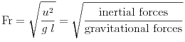
for the Froude number, and

${\rm We}_{{\scriptscriptstyle{\mathbb{W}}}}=\frac{\rho _{{\scriptscriptstyle{\mathbb{W}}}}\; u^{2}\; l}{\sigma _{{{\scriptscriptstyle{\mathbb{O}}}{\scriptscriptstyle{\mathbb{W}}}}}}=\frac{\mbox{inertial forces}}{\mbox{capillary forces}}$

(6.24)

for the Weber number. The corresponding dimensionless ratios for the oil phase are related to those for the water phase as

$\mbox{\rm Re}_{{\scriptscriptstyle{\mathbb{O}}}}=\mbox{\rm Re}_{{\scriptscriptstyle{\mathbb{W}}}}\;\frac{\rho _{{\scriptscriptstyle{\mathbb{O}}}}}{\rho _{{\scriptscriptstyle{\mathbb{W}}}}}\;\frac{\mu _{{\scriptscriptstyle{\mathbb{W}}}}}{\mu _{{\scriptscriptstyle{\mathbb{O}}}}}$

(6.25)

${\rm We}_{{\scriptscriptstyle{\mathbb{O}}}}={\rm We}_{{\scriptscriptstyle{\mathbb{W}}}}\;\frac{\rho _{{\scriptscriptstyle{\mathbb{O}}}}}{\rho _{{\scriptscriptstyle{\mathbb{W}}}}}$

(6.26)

by viscosity and density ratios.

Table IV gives approximate values for densities, viscosities and surface tensions under reservoir conditions [47, 48]. In the following these values will be used to make order of magnitude estimates.

Table IV: Order of magnitude estimates for densities, viscosities and surface tension of oil and water under reservoir conditions

$\rho _{{\scriptscriptstyle{\mathbb{O}}}}$	$\rho _{{\scriptscriptstyle{\mathbb{W}}}}$	$\mu _{{\scriptscriptstyle{\mathbb{O}}}}$	$\mu _{{\scriptscriptstyle{\mathbb{W}}}}$	$\sigma _{{{\scriptscriptstyle{\mathbb{O}}}{\scriptscriptstyle{\mathbb{W}}}}}$
$800\;\mbox{kg}\,\mbox{m}^{{-3}}$	$1000\;\mbox{kg}\,\mbox{m}^{{-3}}$	$0.0018\;\mbox{N}\,\mbox{m}^{{-2}}\,\mbox{s}$	$0.0009\;\mbox{N}\,\mbox{m}^{{-2}}\,\mbox{s}$	$0.035\;\mbox{N}\,\mbox{m}^{{-1}}$

Typical pore sizes in an oil reservoir are of order $l\approx 10^{{-4}}\;\mbox{m}$ and microscopic fluid velocities for reservoir floods range around $u\approx 3\times 10^{{-6}}\;\mbox{m}\,\mbox{s}^{{-1}}$ . Combining these estimates with those of Table IV shows that the dimensionless ratios obey $\mbox{\rm Re}_{{\scriptscriptstyle{\mathbb{O}}}},\mbox{\rm Re}_{{\scriptscriptstyle{\mathbb{W}}}},{\rm Fr}^{2},{\rm We}_{{\scriptscriptstyle{\mathbb{O}}}},{\rm We}_{{\scriptscriptstyle{\mathbb{W}}}}\ll 1$ . Therefore, the pore scale equations (6.16) reduce to the simpler Stokes form

$\begin{array}[]{rcl}0&=&\widehat{\Delta}\widehat{\bf v}_{{\scriptscriptstyle{\mathbb{W}}}}+\frac{\displaystyle 1}{\displaystyle{\rm Gr}_{{\scriptscriptstyle{\mathbb{W}}}}}\;\widehat{\mbox{\boldmath$\nabla$}}\widehat{z}-\frac{\displaystyle 1}{\displaystyle{\rm Ca}_{{\scriptscriptstyle{\mathbb{W}}}}}\;\widehat{\mbox{\boldmath$\nabla$}}\widehat{P}_{{\scriptscriptstyle{\mathbb{W}}}}\\ 0&=&\widehat{\Delta}\widehat{\bf v}_{{\scriptscriptstyle{\mathbb{O}}}}+\frac{\displaystyle 1}{\displaystyle{\rm Gr}_{{\scriptscriptstyle{\mathbb{O}}}}}\;\widehat{\mbox{\boldmath$\nabla$}}\widehat{z}-\frac{\displaystyle 1}{\displaystyle{\rm Ca}_{{\scriptscriptstyle{\mathbb{O}}}}}\;\widehat{\mbox{\boldmath$\nabla$}}\widehat{P}_{{\scriptscriptstyle{\mathbb{O}}}}\end{array}$

(6.27)

where

${\rm Ca}_{{\scriptscriptstyle{\mathbb{W}}}}=\frac{{\rm We}_{{\scriptscriptstyle{\mathbb{W}}}}}{\mbox{\rm Re}_{{\scriptscriptstyle{\mathbb{W}}}}}=\frac{\mbox{viscous forces}}{\mbox{capillary forces}}=\frac{\mu _{{\scriptscriptstyle{\mathbb{W}}}}\; u}{\sigma _{{{\scriptscriptstyle{\mathbb{O}}}{\scriptscriptstyle{\mathbb{W}}}}}}=\frac{u}{u^{*}_{{\scriptscriptstyle{\mathbb{W}}}}}$

(6.28)

is the microscopic capillary number of water, and

${\rm Gr}_{{\scriptscriptstyle{\mathbb{W}}}}=\frac{{\rm Fr}^{2}}{\mbox{\rm Re}}=\frac{\mbox{viscous forces}}{\mbox{gravity forces}}=\frac{\mu _{{\scriptscriptstyle{\mathbb{W}}}}\; u}{\rho _{{\scriptscriptstyle{\mathbb{W}}}}\; g\; l^{2}}$

(6.29)

is the microscopic “gravity number” of water. The capillary number is a measure of velocity in units of

$u^{*}_{{\scriptscriptstyle{\mathbb{W}}}}=\frac{\sigma _{{{\scriptscriptstyle{\mathbb{O}}}{\scriptscriptstyle{\mathbb{W}}}}}}{\mu _{{\scriptscriptstyle{\mathbb{W}}}}}$

(6.30)

a characteristic velocity at which the coherence of the oil-water interface is destroyed by viscous forces. The capillary and gravity numbers for the oil phase can again be expressed through density and viscosity ratios as

$\displaystyle{\rm Ca}_{{\scriptscriptstyle{\mathbb{O}}}}$	$\displaystyle=$	$\displaystyle{\rm Ca}_{{\scriptscriptstyle{\mathbb{W}}}}\;\frac{\mu _{{\scriptscriptstyle{\mathbb{O}}}}}{\mu _{{\scriptscriptstyle{\mathbb{W}}}}}$		(6.31)
$\displaystyle{\rm Gr}_{{\scriptscriptstyle{\mathbb{O}}}}$	$\displaystyle=$	$\displaystyle{\rm Gr}_{{\scriptscriptstyle{\mathbb{W}}}}\;\frac{\rho _{{\scriptscriptstyle{\mathbb{W}}}}}{\rho _{{\scriptscriptstyle{\mathbb{O}}}}}\;\frac{\mu _{{\scriptscriptstyle{\mathbb{O}}}}}{\mu _{{\scriptscriptstyle{\mathbb{W}}}}}.$		(6.32)

Many other dimensionless ratios may be defined. Of general interest are dimensionless space and time variables. Such ratios are formed as

${\rm Gl}_{{\scriptscriptstyle{\mathbb{W}}}}=\frac{{\rm Ca}_{{\scriptscriptstyle{\mathbb{W}}}}}{{\rm Gr}_{{\scriptscriptstyle{\mathbb{W}}}}}=\frac{{\rm We}_{{\scriptscriptstyle{\mathbb{W}}}}}{{\rm Fr}^{2}}=\frac{\mbox{gravity forces}}{\mbox{capillary forces}}=\frac{\rho _{{\scriptscriptstyle{\mathbb{W}}}}\, g\, l^{2}}{\sigma _{{{\scriptscriptstyle{\mathbb{O}}}{\scriptscriptstyle{\mathbb{W}}}}}}=\frac{l^{2}}{l^{{*\, 2}}_{{\scriptscriptstyle{\mathbb{W}}}}}$

(6.33)

which has been called the “gravillary number” [47, 48]. The gravillary number becomes the better known bond number if the density $\rho _{{\scriptscriptstyle{\mathbb{W}}}}$ is replaced with the density difference $\rho _{{\scriptscriptstyle{\mathbb{W}}}}-\rho _{{\scriptscriptstyle{\mathbb{O}}}}$ . The corresponding length

$l^{*}_{{\scriptscriptstyle{\mathbb{W}}}}=\sqrt{\frac{\sigma _{{{\scriptscriptstyle{\mathbb{O}}}{\scriptscriptstyle{\mathbb{W}}}}}}{\rho _{{\scriptscriptstyle{\mathbb{W}}}}\, g}}$

(6.34)

separates capillary waves with wavelengths below $l^{*}_{{\scriptscriptstyle{\mathbb{W}}}}$ from gravity waves with wavelengths above $l^{*}_{{\scriptscriptstyle{\mathbb{W}}}}$ . A dimensionless time variable is formed from the gravillary and capillary numbers as

$\frac{\sqrt{{\rm Gl}_{{\scriptscriptstyle{\mathbb{W}}}}}}{{\rm Ca}_{{\scriptscriptstyle{\mathbb{W}}}}}=\frac{\mbox{\rm Re}_{{\scriptscriptstyle{\mathbb{W}}}}}{{\rm Fr}\,\sqrt{{\rm We}{\scriptscriptstyle{\mathbb{W}}}}}=\frac{(\mbox{gravity f.})^{{3/2}}}{(\mbox{capillary f.})^{{1/2}}\!\times\!\mbox{viscous f.}}=\frac{\sqrt{\rho _{{\scriptscriptstyle{\mathbb{W}}}}\sigma _{{{\scriptscriptstyle{\mathbb{O}}}{\scriptscriptstyle{\mathbb{W}}}}}g}\, t}{\mu _{{\scriptscriptstyle{\mathbb{W}}}}}=\frac{t}{t^{*}_{{\scriptscriptstyle{\mathbb{W}}}}}$

(6.35)

where

$t^{*}_{{\scriptscriptstyle{\mathbb{W}}}}=\frac{l^{*}_{{\scriptscriptstyle{\mathbb{W}}}}}{u^{*}_{{\scriptscriptstyle{\mathbb{W}}}}}=\frac{\mu _{{\scriptscriptstyle{\mathbb{W}}}}}{\sqrt{\sigma _{{{\scriptscriptstyle{\mathbb{O}}}{\scriptscriptstyle{\mathbb{W}}}}}\,\rho _{{\scriptscriptstyle{\mathbb{W}}}}\, g}}$

(6.36)

is a characteristic time after which the influence of gravity dominates viscous and capillary effects. The reader is cautioned not to misinterpret the value of $t^{*}_{{\scriptscriptstyle{\mathbb{W}}}}$ in Table V below as an indication that gravity forces dominate on the pore scale.

Table V collects definitions and estimates for the dimensionless groups and the numbers $l^{*},u^{*}$ and $\nu^{*}$ characterizing the oil-water system.

Table V: Overview of definitions and estimates for characteristic microscopic numbers describing oil and water flow under reservoir conditions

Quantity	Definition	Estimate
$\mbox{\rm Re}_{{\scriptscriptstyle{\mathbb{W}}}}$	$\frac{\displaystyle\rho _{{\scriptscriptstyle{\mathbb{W}}}}\; u\; l}{\displaystyle\mu _{{\scriptscriptstyle{\mathbb{W}}}}}$	$3.3\cdot 10^{{-4}}$
${\rm Ca}_{{\scriptscriptstyle{\mathbb{W}}}}$	$\frac{\displaystyle\mu _{{\scriptscriptstyle{\mathbb{W}}}}\; u}{\displaystyle\sigma _{{{\scriptscriptstyle{\mathbb{O}}}{\scriptscriptstyle{\mathbb{W}}}}}}$	$7.7\cdot 10^{{-8}}$
${\rm Gr}_{{\scriptscriptstyle{\mathbb{W}}}}$	$\frac{\displaystyle\mu _{{\scriptscriptstyle{\mathbb{W}}}}\; u}{\displaystyle\rho _{{\scriptscriptstyle{\mathbb{W}}}}\; g\; l^{2}}$	$2.8\cdot 10^{{-5}}$
${\rm Gl}_{{\scriptscriptstyle{\mathbb{W}}}}$	$\frac{\displaystyle\rho _{{\scriptscriptstyle{\mathbb{W}}}}\, g\, l^{2}}{\displaystyle\sigma _{{{\scriptscriptstyle{\mathbb{O}}}{\scriptscriptstyle{\mathbb{W}}}}}}$	$2.8\cdot 10^{{-3}}$
$\nu^{*}_{{\scriptscriptstyle{\mathbb{W}}}}$	$\frac{\displaystyle\mu _{{\scriptscriptstyle{\mathbb{W}}}}}{\displaystyle\rho _{{\scriptscriptstyle{\mathbb{W}}}}}$	$9\cdot 10^{{-7}}\;\mbox{m}^{2}\,\mbox{s}^{{-1}}$
$u^{*}_{{\scriptscriptstyle{\mathbb{W}}}}$	$\frac{\displaystyle\sigma _{{{\scriptscriptstyle{\mathbb{O}}}{\scriptscriptstyle{\mathbb{W}}}}}}{\displaystyle\mu _{{\scriptscriptstyle{\mathbb{W}}}}}$	$38.9\;\mbox{m}\,\mbox{s}^{{-1}}$
$l^{*}_{{\scriptscriptstyle{\mathbb{W}}}}$	$\sqrt{\frac{\displaystyle\sigma _{{{\scriptscriptstyle{\mathbb{O}}}{\scriptscriptstyle{\mathbb{W}}}}}}{\displaystyle\rho _{{\scriptscriptstyle{\mathbb{W}}}}\, g}}$	$1.9\;\mbox{cm}$
$t^{*}_{{\scriptscriptstyle{\mathbb{W}}}}$	$\frac{\displaystyle\mu _{{\scriptscriptstyle{\mathbb{W}}}}}{\sqrt{\displaystyle\sigma _{{{\scriptscriptstyle{\mathbb{O}}}{\scriptscriptstyle{\mathbb{W}}}}}\,\rho _{{\scriptscriptstyle{\mathbb{W}}}}\, g}}$	$4.9\cdot 10^{{-4}}\;\mbox{s}$

For these estimates the values in Table IV together with the above estimates of $l$ and $u$ have been used. Table V shows that

$\mbox{viscous forces}\ll\mbox{gravity forces}\ll\mbox{capillary forces},$

(6.37)

and hence capillary forces dominate on the pore scale [333, 2, 47, 48].

From the Stokes equation (6.27) it follows immediately that for low capillary number floods ( ${\rm Ca}\ll 1$ ) the viscous term as well as the shear term in the boundary condition (6.20) become negligible. Therefore the velocity field drops out, and the problem reduces to finding the equilibrium capillary pressure field. The equilibrium configuration of the oil-water interface then defines timeindependent pathways for the flow of oil and water. Hence, for flows with microscopic capillary numbers ${\rm Ca}\ll 1$ an improved methodology for a quantitative description of immiscible displacement from pore scale physics requires improved calculations of capillary pressures from the pore scale, and much research is devoted to this topic [347, 348, 246a].

Author:	R. Hilfer
originally published in:	Advances in Chemical Physics 92, 299-424 (1996)
originally submitted:	May 9th, 1995