4 Approximate Analytical Solution

[2330.2.1] The basic idea of the analysis below is to approximate the travelling wave profile for long times t→∞ with piecewise constant functions (step functions). [2330.2.2] For large [page 2331, §0]    Ca→∞ (i.e. in the Buckley-Leverett limit) one may view this approximate profile as a superposition of two Buckley-Leverett shock fronts. [2331.0.1] This is possible by virtue of the fact, that the Heaviside step function

can also be regarded as a function of the similarity variable z/t of the Buckley-Leverett problem.

[2331.1.1] In the crudest approximation one can split the total profile for sufficiently large t into the sum

of an imbibition front

located at zim=c*⁢t+z* and a drainage front profile located at zdr=c*⁢t

both moving with the same speed c*, where Sin=s⁢-∞ resp. Sout=s⁢∞ are the upper (inlet) resp. lower (outlet) saturations and S* is the maximum (overshoot) saturation. [2331.1.2] The quantity z*=zim-zdr is the distance by which the imbibition front precedes the drainage front, i.e. the width of the tip (=overshoot) region.

[2331.2.1] The two equations (28) become coupled, if eq.  (20) holds true, because then there is only a single wave speed c* for both fronts. [2331.2.2] At the imbibition discontinuity the Rankine-Hugoniot condition demands

and the second equality (with colon) defines the function cim⁢S. [2331.2.3] Similarly

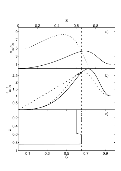
defines the drainage front velocity as a function cdr⁢S of the overshoot S*. Examples of the velocities ci used in the compuations are shown in Figure 1a. [2331.2.4] For a travelling wave both fronts move with the same velocity so that the mathematical problem is to find a solution S* of the equation

obtained from equating eqs. (37b) and (37a) (See Fig. 1a). [2331.2.5] The wave velocity c* is then obtained as cim⁢S* or equivalently as cdr⁢S*.

[page 2332, §1]

[2332.1.1] Equation (38) provides a necessary condition for the existence of a travelling wave solution of the form of eq.  (36) with velocity c* and overshoot S*. [2332.1.2] More generally, if the saturation plateau SP is larger or smaller than S*, one expects to find non-monotone profiles that are, however, not travelling waves. [2332.1.3] Instead the drainage and imbibition fronts are expected to have different velocities. [2332.1.4] The fractional flow functions with relative permeabilities from eqs. (31) and the parameters from Table 1 give for SP<S* the result

while for SP>S* one has

[2332.1.5] In this case, for plateau saturations SP<S*, the leading (imbibition) front has a smaller velocity than the trailing (drainage) front. [2332.1.6] Thus the trailing front catches up and the profile approaches a single front at long times. [2332.1.7] For plateau saturations SP>S* on the other hand the trailing drainage front moves slower than the leading imbibition front. [2332.1.8] In this case a non-monotone profile persists indefinitely, albeit with a plateau (tip) width that increases linearly with time.