3.1 Complex Zeros
[642.2.1] Contrary to the exponential function the Mittag-Leffler functions
exhibit complex zeros denoted as z0.
[642.2.2] The complex zeros were studied by Wiman [8] who
found the asymptotic curve along which the zeros
are located for 0<α<2 and showed that
they fall on the negative real axis for all α≥2.
[642.2.3] For real α,β these zeros come in complex conjugate pairs.
[642.2.4] The pairs are denoted as zk0α with integers k∈Z
where k>0 (resp. k≤0) labels zeros in the upper (resp. lower) half plane.
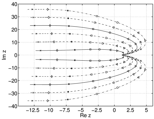
[642.2.5] Figure 1 shows lines that the complex zeros
zk0α, k=-5,…,6 of Eα,1z trace out as functions
of α for 0.1≤α≤0.99995.
[642.2.6] Figure 1 gives strong
numerical evidence that the distance between
zeros diminishes as α→0.
[642.2.7] Moreover all zeros approach the point z=1 as α→0.
[642.2.8] This fact seems to have been overlooked until now.
[642.2.9] Of course, for every fixed α>0 the point z=1 is neither
a zero nor an accumulation point of zeros
because the zeros of an entire function must remain isolated.
[642.2.10] The numerical evidence is confirmed analytically.
Theorem 3.1.
The zeros zk0α of Eα,1z obey
for all k∈Z.
[643.0.1] For the proof we note that Wiman showed [8, p. 226]
| limk→∞argz±k0α=±απ2 | | (35) |
and further that the number
of zeros with zk0<r is given by
r1/α/π-1+α/2 [8, p. 228].
[643.0.2] From this follows that
| 1-α2απα<zk0α<2k+1-α2απα | | (36) |
for all k∈Z.
[643.0.3] Taking the limit α→0 in (35) and (36)
gives zk0=1 and argzk0=0 for all k∈Z.
[page 644, §1]
[644.1.1] The theorem states that in the limit α→0
all zeros collapse into a singularity at z=1.
[644.1.2] Next we turn to the limit α→1.
[644.1.3] Of course for α=1 we have E1,1z=expz
which is free from zeros.
[644.1.4] Figure 1 shows that this is indeed
the case because, as α→1, the zeros approach -∞
along straight lines parallel to the negative real axis.
[644.1.5] In fact we find
Theorem 3.2.
Let ϵ>0.
Then the zeros zk0α of Eα,1z obey
| limϵ→0Imzk01-ϵ | =2k-1π | | (37) |
| limϵ→0Imzk01+ϵ | =2kπ | | (38) |
for all k∈Z.
[644.1.6] The theorem shows that the phase switches
as α crosses the value α=1
in the sense that minima (valleys)
and maxima (hills) of the Mittag-Leffler
function are exchanged
(see also Figures 7 and
8 below).
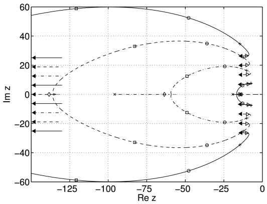
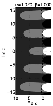
[644.2.1] The location of zeros as function of α for the
case 1<α<2 is illustrated in Figure 2.
[644.2.2] Note that with increasing α more and more pairs of
zeros collapse onto the negative real axis.
[644.2.3] The collapse appears to happen in a continuous manner
(see also Figures 9 and 10
below).
[644.2.4] It is interesting to note that after two conjugate zeros
merge to become a single zero on the negative real axis
this merged zero first moves to the right towards zero and
only afterwards starts to move left towards -∞.
[644.2.5] This effect can also be seen in Figure 2.
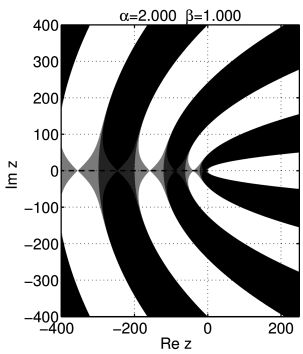
[644.2.6] For α=2 the zeros -k-1/22π2 all fall
on the negative real axis as can be seen
in Figure 11 below.
[644.2.7] For α>2 all zeros lie on the negative real axis.
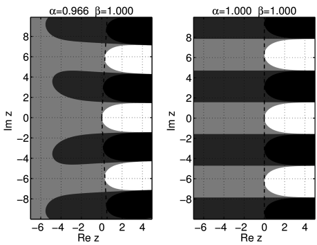
3.2 Contour Lines
[644.3.1] Next we present contour plots for ReEα,βz.
[644.3.2] We use the notation
| Cα,βRev | =z∈C:ReEα,βz=v | | (39) |
| Cα,βImv | =z∈C:ImEα,βz=v | | (40) |
for the contour lines of the real and imaginary part.
[644.3.3] The region z∈C:ReEα,βz>1 will be coloured white.
[644.3.4] The region z∈C:ReEα,βz<-1 will be coloured black.
[644.3.5] The region z∈C:0≤ReEα,βz≤1 is light gray.
[644.3.6] The region z∈C:-1≤ReEα,βz≤0 is dark gray.
[644.3.7] Thus the contour line Cα,βRe0 separates the light gray from dark
gray, the contour Cα,βRe1 separates white from light gray,
and Cα,βRe-1 dark gray from black.
[644.3.8] Because ReEα,βz is continuous there exists
in all figures light and dark gray regions between white
and black regions even if the gray regions
cannot be discerned on a figure.
[page 645, §1]
[645.1.1] We begin our discussion with the case α→0.
Setting α=0 the series (1) defines the function
for all z<1.
[645.1.2] This function is not entire, but can be analytically
continued to all of C∖1, and
has then a simple pole at z=1 for all β.
[645.1.3] In Figure 3 we show the contour plot
for the case α=0, β=1.
[645.1.4] The contour line C0,1Re0 is the straight line
Rez=1 separating the left and right half plane.
[645.1.5] The contour line C0,1Re1 is the boundary circle
of the white disc on the left, while the contour line
C0,1Re-1 is the boundary of the black disc on the right.
[645.2.1] Having discussed the case α=0 we turn
to the case α>0 and note that the limit
α→0 is not continuous.
[645.2.2] For α>0 the Mittag-Leffler function is an entire function.
[645.2.3] As an example we show the contour plot for α=0.2, β=1
in Figure 4.
[645.2.4] The central white circular lobe extending
[page 646, §0]
to the origin appears to be a remnant of the white disc
in Figure 3.
[646.0.1] They evolve continuously from each other
upon changing α between 0 and 0.2.
[646.0.2] It seems as if the singularity at z=1
for α=0 had moved along the real axis through the black
circle to ∞ thereby producing an infinite number of
secondary white and black lobes (or fingers) confined to a
wedge shaped region with opening angle απ/2.
[646.1.1] The behaviour of Eα,βz for 0<α<2 is generally
dominated by the wedge W+απ/2
indicated by dashed lines in Figure 4.
[646.1.2] For z∈W+απ/2 the Mittag-Leffler
function grows to infinity as z→∞.
[646.1.3] Inside this wedge the function oscillates as a
function of Imz.
[646.1.4] For z∈W-απ/2 the function decays to zero as
z→∞.
[646.1.5] Along the delimiting rays, i.e. for argz=±απ/2,
the function approaches 1/α in an oscillatory fashion.
[646.2.1] The oscillations inside the wedge are seen as black and
white lobes (or fingers) in Figure 4.
[646.2.2] Each white finger is surrounded by a light gray region.
[646.2.3] Near the tip of the light gray region surrounding a white
finger lie complex zeros of the Mittag-Leffler function.
[646.2.4] The real part ReEα,βz
is symmetric with respect to the real axis.
[646.3.1] Contrary to C0,1Re0 the contour line C0.2,1Re0
consists of infinitely many pieces.
[646.3.2] These pieces will be denoted as
C0.2,1Re0;±k with k=1,2,3,… located in the
upper (+) resp. lower (-) half plane.
[646.3.3] The numbering is chosen from left to right, so that
C0.2,1Re0;±1 separates the light gray region
in the left half plane from the dark gray in the right half plane.
[646.3.4] The line C0.2,1Re0;+2 is the boundary of the
light gray region surrounding the first white “finger”
(lobe) in the upper half plane and C0.2,1Re0;-2
is its reflection on the real axis.
[646.3.5] Similarly for k=3,4,….
[646.3.6] Note that C0.2,1Re0;±1 seem to encircle the
central white lobe (“bubble”) by going to ±i∞ parallel to the
imaginary axis.
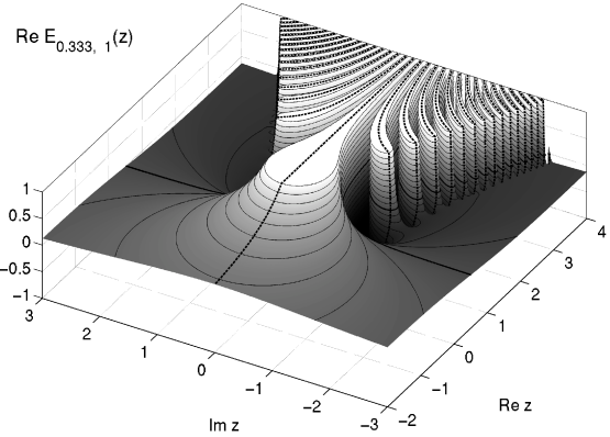
[646.4.1] With increasing α the wedge W+απ/2 opens,
the central lobe becomes smaller, the side fingers (or lobes)
grow thicker and begin to extend towards the left half plane.
[646.4.2] At the same time the contour line Cα,1Re0;±1 moves
to the left.
[646.4.3] This is illustrated in a threedimensional plot of
ReE0.333,1z in Figure 5.
[646.4.4] In this Figure we have indicated also the complex zeros
as the intersection of C0.333,1Re0 (shown as thick
solid lines) and C0.333,1Im0 (shown as thick
dashed lines).
[646.4.5] At α=1/2 the contours C0.5,1Re0;±1 cross
the imaginary axis.
[page 647, §1]
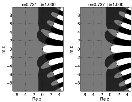
[647.1.1] Around α≈0.73 the contours Cα,1Re0;±2
osculate the contours Cα,1Re0;±1.
[647.1.2] The osculation eliminates a light gray finger and creates
a dark gray finger.
[647.1.3] In Figure 6
we show the situation before and after the osculation.
[647.1.4] This is the first of an infinity of similar osculations
between Cα,1Re0;±1 and Cα,1Re0;±k
for k=2,3,4,….
[647.1.5] We estimate the value of α for the first
osculation at α≈0.734375±0.000015.
[647.2.1] For α→1 the dark gray fingers (where ReEα,β<0)
extend more and more into the left half plane.
[647.2.2] For α=1 the wedge W+π/2 becomes the right half plane
and the lobes or fingers run parallel to the real axis.
[647.2.3] The dark gray fingers, and therefore the oscillations,
now extend to -∞.
[647.2.4] The contour lines C1,1Re0;±k degenerate into
| C1,1Re0;±k=z∈C:Imz=±kπ/2,k=1,2,3,… | | (42) |
i.e. into straight lines parallel to the real axis.
[647.2.5] This case is shown in Figure 7.
[647.2.6] For α=1+ϵ with ϵ>0 the gray
fingers are again finite.
[647.2.7] This is shown in Figure 8.
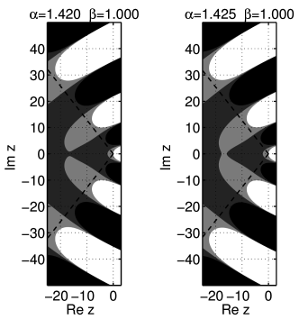
[647.3.1] As α is increased further the fingers grow thicker
and approach each other near the negative real axis.
[647.3.2] For α≈1.42215±0.00005 the first of an infinite
cascade of osculations appears.
[647.3.3] This is shown in Figure 9.
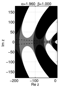
[647.3.4] The limit α→2 is illustrated in
Figures 10 and 11.
[647.3.5] Note that the background colour changes from light
gray in Figure 10 to dark gray in
11 in agreement with the discussion
of complex zeros above.
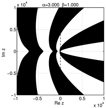
[647.4.1] For α>2 the behaviour changes drastically.
[647.4.2] Figure 12 shows the contour
plot for α=3, β=1.
[647.4.3] Note the scale of the axes and hence there
are no visible dark or light gray regions.
[647.4.4] The wedge shaped region is absent.
[647.4.5] The rays delimiting the wedge may still be
viewed as if the fingers were following them
in the same way as for α<2.
[647.4.6] Thus the fingers are more strongly bent
as they approach the negative real axis.
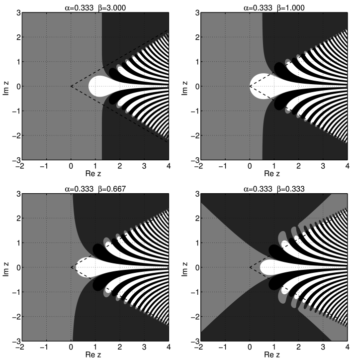
[647.5.1] Now we turn to the cases β≠1 choosing α=1/3
for illustration.
[647.5.2] For β>1 equation (41) implies that
the central lobe first grows (because Γβ diminishes)
and then shrinks as β→∞ for small values of α.
[647.5.3] This is illustrated in the upper left subfigure of
Figure 13.
[647.5.4] For reference the case β=1 is also shown
in the upper right subfigure of Figure 13.
[647.6.1] More interesting behaviour is obtained for β<1.
[647.6.2] In this case the contours C1/3,βRe0;±1
stop to run to infinity parallel to the imaginary axis.
[647.6.3] Instead they seem to approach infinity along rays
extending into the negative half axis as illustrated
in the lower left subfigure of Figure 13.
[647.6.4] At the same time a sequence of osculations between
C1/3,βRe0;±k and C1/3,βRe0;±k+1
begins starting from k=∞.
[647.6.5] One of the last of these osculations can be
seen for β=1/3 on the lower right subfigure of
Figure 13.
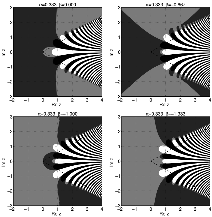
[647.6.6] As β falls below 1/3 the contour C1/3,βRe0;+1
coalesces with C1/3,βRe0;-1 to form a new large
finite central lobe.
[647.6.7] This new second lobe becomes smaller and retracts towards
the origin for β→0.
[647.6.8] This can be seen from the upper left subfigure of
Figure 14 where the case β=0
is shown.
[647.6.9] As β falls below zero the same process of formation
of a new central lobe accompanied by a cascade of
osculations starts again.
[647.6.10] This occurs iteratively whenever β crosses a negative
integer and is a consequence of the poles in Γβ.