Article

[page 2297, §1]
[2297.1.1] Amorphous polymers and supercooled liquids near the glass transition temperature exhibit strongly nonexponential response and relaxation functions in various experiments [10]. [2297.1.2] Dielectric spectroscopy experiments show an asymmetrically broadened relaxation peak, often called $\alpha$ -relaxation peak, that flattens into an excess wing at high frequencies [9, 11].

[2297.2.1] Most theoretical and experimental works use a small number of empirical expressions such as the formulae of Cole-Davidson (CD) [2], Havriliak-Negami (HN) [8] or Kohlrausch-Williams-Watts (KWW) [13] for fitting of the asymmetric $\alpha$ -relaxation peak. [2297.2.2] All of these phenomenological fitting formulae are obtained by the method of introducing a fractional “stretching” exponent into the standard Debye relaxation in the time or frequency domain. [2297.2.3] In the frequency domain the relaxation is described in terms of a normalized complex susceptibility

$\widehat{\chi}(u)=\frac{\chi(\omega)-\chi _{\infty}}{\chi _{0}-\chi _{\infty}}$

(1)

where $u=-\mbox{i}\omega$ , $\omega$ is the circular frequency, $\chi(\omega)$ is a dynamic susceptibility normalized by the corresponding isothermal susceptibility, $\chi _{0}=\lim _{{\omega\to 0}}\operatorname{Re}\chi(\omega)$ is the static susceptibility, and $\chi _{\infty}=\lim _{{\omega\to\infty}}\operatorname{Re}\chi(\omega)$ gives the “instantaneous” response. [2297.2.4] Of course, for dielectric relaxation [page 2298, §0] experiments $\chi$ is just the complex frequency dependent dielectric susceptibility (often denoted by $\varepsilon$ ), and the the more general notation $\chi$ is used as a reminder that the same expressions apply for other relaxation experiments such as e.g. for mechanical relaxation. [2298.0.1] Relaxation in the time domain is described by a normalized relaxation function $f(t)$ defined as

$f(t)=\begin{cases}\phi(t)/\phi(0)&\text{for }t\geq 0\\ 0&\text{for }t<0.\end{cases}$

(2)

where $\phi(t)$ denotes an experimental relaxation function (such as e.g. the electrical polarization in dielectric experiments) normalized by the isothermal susceptibility $\phi(0)=\chi _{0}-\chi _{\infty}$ . [2298.0.2] Experiments in the time domain measuring $f(t)$ are related to experiments in the frequency domain measuring $\operatorname{Re}\widehat{\chi}(u)$ (or $\operatorname{Im}\widehat{\chi}(u)$ ) through the formula

$\widehat{\chi}(u)=1-u\;{\mathcal{L}}\left\{ f(t)\right\}(u)$

(3)

where ${\mathcal{L}}\left\{ f(t)\right\}(u)$ is the Laplace transform of the relaxation function $f(t)$ . [2298.0.3] Modern broadband dielectric spectroscopy [12] utilizes time and frequency domain measurements simultaneously.

[2298.1.1] Dielectric loss spectra very often show a marked excess contribution at frequencies some decades above the peak frequency of the $\alpha$ -relaxation [9]. [2298.1.2] Experimentally this so called excess wing was already noted in the early works [2], but until today there is no commonly accepted model for the microscopic origin of the excess wing in glass forming materials. [2298.1.3] It is therefore the objective of this short communication to note that there exists a simple fit formula involving only a single stretching exponent that seems to fit the excess wing better than the traditional fit functions.

[2298.2.1] Given the objective of introducing an improved phenomenological fit function it is pertinent to list first the traditional formulae against which to compare the new proposal. [2298.2.2] Let me begin with the three-parameter formula for a two-step Debye relaxation

$\widehat{\chi}(u)=\frac{1+u{\tau}_{2}(1-C)}{(1+u{\tau}_{1})(1+u{\tau}_{2})}$

(4)

where $0<{\tau}_{1}<{\tau}_{2}<\infty$ are the two relaxation times and $C$ is a parameter that fixes the relative dielectric strength of the two relaxation processes. [2298.2.3] Of course this formula is equivalent to the popular relaxation time distribution model

$\widehat{\chi}(u)=\int _{0}^{\infty}\frac{p({\tau})}{(1+{\tau}u)}\mbox{\rm d}{\tau}$

(5)

with a sum of two $\delta$ -distributions for the probability density function of relaxation times ( $0<{\tau}_{1}<{\tau}_{2}<\infty$ )

$p({\tau})=\left(1-\frac{C}{1-({\tau}_{1}/{\tau}_{2})}\right)\delta({\tau}-{\tau}_{1})+\left(\frac{C}{1-({\tau}_{1}/{\tau}_{2})}\right)\delta({\tau}-{\tau}_{2}).$

(6)

[2298.2.4] Relaxation time distributions with more parameters will give better fits at the expense of introducing more parameters, but here attention will be restricted to fit functions with two or three parameters. [2298.2.5] In Reference [3] Davidson and Cole discussed the two-parameter expression

$\widehat{\chi}(u)=\frac{1}{(1+u{\tau _{{\gamma}}})^{{\gamma}}},\quad 0<{\gamma}\leq 1,$

(7)

for the normalized susceptibility containing a single stretching exponent $0<{\gamma}\leq 1$ and single relaxation time constant $0<{\tau _{{\gamma}}}<\infty$ . [2298.2.6] Another popular three-parameter fitting formula for the frequency dependent susceptibility was discussed by Havriliak-Negami [8]

$\widehat{\chi}(u)=\frac{1}{(1+(u{\tau _{{H}}})^{{\alpha}})^{{\gamma}}}$

(8)

[page 2299, §0] with two stretching exponents $0<{\alpha},{\gamma}\leq 1$ and one relaxation time $0<{\tau _{{H}}}<\infty$ . [2299.0.1] Many works on dielectric relaxation utilize also the earlier Cole-Cole formula [1] (obtained by setting ${\gamma}=1$ in equation (8)) but note that this yields a symmetrically broadened peak in contrast with most experimental observations on $\alpha$ -peaks.

[2299.1.1] All of the fitting formulae above were defined in the frequency domain. They can be transformed into the time domain using equation (3). [2299.1.2] A widely used fitting formula in the time domain, on the other hand, is the stretched exponential relaxation function

$f(t)=\exp[-(t/{\tau _{{\beta}}})^{{\beta}}],\quad 0<{\beta}\leq 1,$

(9)

with exponent $0<{\beta}\leq 1$ and time constant ${\tau _{{\beta}}}$ [13]. [2299.1.3] The stretched exponential relaxation function can be transposed to the frequency domain using (3). [2299.1.4] One obtains for the susceptibility the little known result

$\widehat{\chi}(u)=1-H_{{\beta}}(-(u{\tau _{{\beta}}})^{{\beta}})$

(10)

where $H_{{\beta}}$ is defined by the series

$H_{{\beta}}(x)=\sum _{{k=0}}^{\infty}\frac{\Gamma({\beta}k+1)}{\Gamma(k+1)}x^{{-k}}$

(11)

[page 2300, §0] convergent for all $0<x<\infty$ . [2300.0.1] This Kohlrausch susceptibility function was recently discussed in Ref. [7] together with the time domain relaxation functions corresponding to the Havriliak-Negami susceptibility and its special cases in terms of $H$ -functions.

[2300.1.1] The main purpose of this short letter is to introduce a simple three-parameter fit function that seems to work well not only for fitting to the asymmetric $\alpha$ -peak, but also for the excess wing at high frequency. [2300.1.2] The functional form is

$\widehat{\chi}(u)=\frac{1+({\tau _{{\alpha}}}u)^{{\alpha}}}{1+(u{\tau _{{\alpha}}})^{{\alpha}}+u{\tau^{{\,\prime}}_{{\alpha}}}}$

(12)

containing a single stretching exponent $0<{\alpha}\leq 1$ and relaxation times $0<{\tau _{{\alpha}}},{\tau^{{\,\prime}}_{{\alpha}}}<\infty$ . [2300.1.3] The functional form was obtained from the theory of fractional dynamics [5, 4, 6], but this fact is not important in the present context. [2300.1.4] Rather it is the purpose here to compare the new function with the traditional functions on the level of a phenomenological fitting function.

[2300.2.1] The results are presented for the broadband dielectric spectra of glass forming propylene carbonate reported in [12]. [2300.2.2] At a temperature of $T=193$ K the dielectric spectrum shows a broadened $\alpha$ -peak and excess high frequency wing over roughly 5 decades in frequency. [2300.2.3] The data are then fitted simultaneously for the real and imaginary part. [2300.2.4] The fit uses only data from three decades (from $f=10^{{5.1}}$ Hz to $f=10^{{8.1}}$ Hz) around the maximum of the imaginary part as indicated by vertical dashed lines in the figure. [2300.2.5] The two-step Debye fit uses equation (4), the [page 2301, §0] Cole-Davidson (CD) fit uses (7), the Havriliak-Negami (HN) fit uses (8), the Kohlrausch-Williams-Watts (KWW) fit uses (10) and the fractional dynamics (FD) fit uses equation (12). [2301.0.1] In all fits an additional fit parameter is the isothermal susceptibility $\phi(0)=\chi _{0}-\chi _{\infty}$ .

[2301.1.1] Figure 1 shows the results for the real part. [2301.1.2] The data have been displaced in the vertical direction from their original location corresponding to FD in order to better distinguish the quality of the different fits.

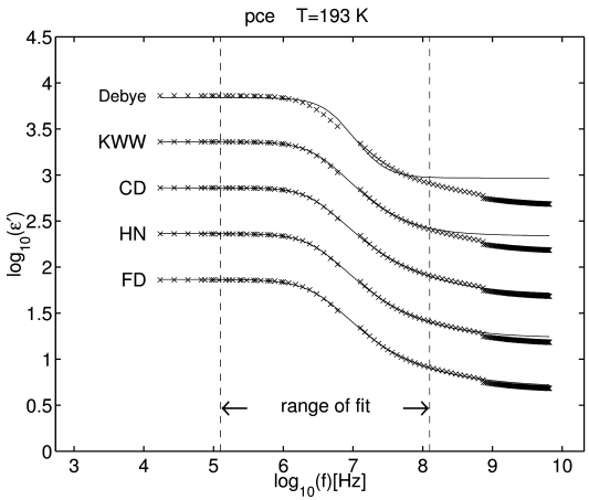
Figure 1: Five different fits to the real part $\varepsilon^{\prime}(f)=\operatorname{Re}\chi(u)$ ( $u=-2\pi\mbox{i}f$ ) of the complex dielectric function of propylene carbonate at $T=193K$ as a function of frequency $f$ . Experimental data represented by crosses are taken from Ref. [12]. The fitting function is given by equation (1) combined with eq. (4) (Debye), eq. (7) (CD), eq. (8) (HN), eq. (10) (KWW), and eq. (12) (FD), The range over which the data were fitted is indicated by dashed vertical lines in the figure. For clarity the data were displaced vertically by half a decade each. The original location of the data corresponds to the curve labelled FD.

[2301.1.3] Clearly the two-step Debye fit is not as good as the other fits in the fitting range. [2301.1.4] Extending the fitting range shows that also the KWW-formula gives not as good agreement as the CD-, HN-, and FD-fits. [2301.1.5] This can also be seen from the fact that the latter fits extend beyond the original fitting range.

[2301.2.1] Figure 2 shows the results for the imaginary part. [2301.2.2] The CD- and HN-fits are seen to be of equal quality. [2301.2.3] They deviate significantly from the experimental data in the excess wing region outside the fitting range. [2301.2.4] Extending the fit range for the CD- and HN-fits would give poorer agreement and systematic deviations around the main peak.

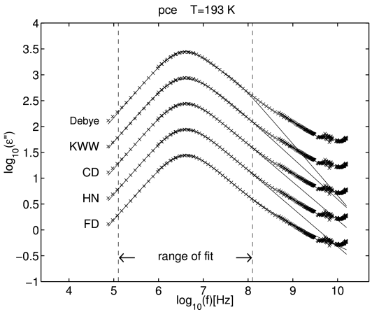
Figure 2: Five different fits to the imaginary part $\varepsilon^{{\prime\prime}}(f)=\operatorname{Im}\chi(u)$ ( $u=-2\pi\mbox{i}f$ ) of the complex dielectric function of propylene carbonate at $T=193K$ as a function of frequency $f$ . Experimental data represented by crosses are taken from Ref. [12]. The fitting function is given by equation (1) combined with eq. (4) (Debye), eq. (7) (CD), eq. (8) (HN), eq. (10) (KWW), and eq. (12) (FD). The range over which the data were fitted is indicated by dashed vertical lines in the figure. For clarity the data were displaced vertically by half a decade each. The original location of the data corresponds to the curve labelled FD.

[2301.2.5] Contrary to the CD- and HN-fits the FD-fit extends well beyond the fitting range into the region of the excess wing. [2301.2.6] Extending the fit range in this case would not lower the quality of the fit near the main peak.

[2301.3.1] In summary the present paper has shown that a simple functional form allows to fit an asymmetrically broadened relaxation peak well into the excess wing. [2301.3.2] Similar to the Cole-Davidson or the Kohlrausch susceptibilities but contrary to the Havrialiak-Negami function and contrary to a combination of Cole-Davidson and Cole-Cole fits[11] the new function requires only a single stretching exponent.

Authors:	R. Hilfer und N.B. Wilding
originally published in:	Journal of Physics C: Condensed Matter, Vol. 14, pages 2297-2301 (2002)
originally submitted:	November 22nd, 2001