4.1 Description of Experimental Sample
[218.0.2] The experimental sample, denoted as SEX, is a
threedimensional microtomographic
image of Fontainebleau sandstone.
[218.0.3] This sandstone is a popular reference standard because of its
chemical, crystallographic and microstructural simplicity
[14, 13].
[218.0.4] Fontainebleau sandstone consists of monocrystalline quartz
grains that have been eroded for long periods before being
deposited in dunes along the sea shore during the Oligocene,
roughly 30 million years ago.
[218.0.5] It is well sorted containing grains of around
200μm
in diameter.
[218.0.6] The sand was cemented by silica crystallizing around the grains.
[218.0.7] Fontainebleau sandstone exhibits intergranular porosity ranging
from 0.03 to roughly 0.3 [13].
Table 2: Overview of geometric properties of the four microstructures
displayed in Figures
1 through
4
| Properties |
SEX |
SDM |
SGF |
SSA |
| M1 |
300 |
255 |
256 |
256 |
| M2 |
300 |
255 |
256 |
256 |
| M3 |
299 |
255 |
256 |
256 |
| ϕP∩S |
0.1355 |
0.1356 |
0.1421 |
0.1354 |
| ϕ2P∩S |
10.4 mm-1 |
10.9 mm-1 |
16.7 mm-1 |
11.06 mm-1 |
| L* |
35 |
25 |
23 |
27 |
| 1-λc0.1355,L* |
0.0045 |
0.0239 |
0.3368 |
0.3527 |
[218.1.1] The computer assisted microtomography was carried out on a
micro-plug drilled from a larger original core.
[218.1.2] The original core from which the micro-plug was taken had a measured
porosity of 0.1484, permability of 1.3D and
formation factor 22.1.
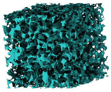
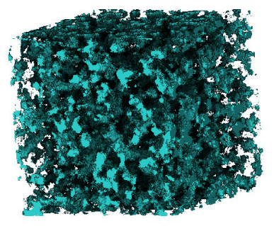
[218.1.3] The porosity ϕSEX of the microtomographic data set
is only 0.1355 (see Table 2).
[218.1.4] The difference between the porosity of the original core and that
of the final data set is due to the heterogeneity of the sandstone and
to the difference in sample size.
[218.1.5] The experimental sample is referred to as EX in the
following.
[218.1.6] The pore space of the experimental sample is visualized
in Figure 1.
4.2 Sedimentation, Compaction and Diagenesis Model
[220.1.1] Fontainebleau sandstone is the result of complex physical,
chemical and geological processes known as sedimentation,
compaction and diagenesis.
[220.1.2] It is therefore natural to model these processes directly
rather than trying to match general geometrical characteristics.
[220.1.3] This conclusion was also obtained from local porosity
theory for the cementation index in Archie’s law
[27].
[220.1.4] The diagenesis model abbreviated as DM in the following,
attempts model the main geological sandstone-forming processes
[4, 48].
[220.2.1] In a first step porosity,
grain size distribution, a visual estimate of the degree of
compaction, the amount of quartz cement and clay contents
and texture are obtained by image analysis of backscattered
electron/cathodo-luminescence images made from thin sections.
[220.2.2] The sandstone modeling is then carried out in three main steps:
grain sedimentation, compaction and diagenesis described in
detail in [4, 48].
[220.3.1] Sedimentation begins by measuring the grain size
distribution using an erosion-dilation algorithm.
[220.3.2] Then spheres with random diameters are
picked randomly according to the grain size distribution.
[220.3.3] They are dropped onto the grain bed and relaxed
into a local potential energy minimum or, alternatively,
into the global minimum.
[220.4.1] Compaction occurs because the sand becomes buried into
the subsurface.
[220.4.2] Compaction reduces the bulk volume (and porosity).
[220.4.3] It is modelled as a linear process in which the vertical coordinate
of every sandgrain is shifted vertically downwards by an amount
proportional to the original vertical position.
[220.4.4] The proportionality constant is called the compaction factor.
[220.4.5] Its value for the Fontainebleau sample is estimated to be
0.1 from thin section analysis.
[220.5.1] In the diagenesis part
only a subset of known diagenetical processes are simulated,
namely quartz cement overgrowth and precipitation of authigenic
clay on the free surface.
[220.5.2] Quartz cement overgrowth is modeled by radially enlarging each grain.
[220.5.3] If R0 denotes the radius of the originally deposited spherical
grain, its new radius along the direction r from grain center
is taken to be [59, 48]
| Rr=R0+minbℓrγ,ℓr | | (59) |
where ℓr is the distance between the surface of the
original spherical grain and the surface of its Voronoi
polyhedron along the direction r.
[220.5.4] The constant b controls the amount of cement, and the
growth exponent γ controls the type of cement overgrowth.
[220.5.5] For γ>0 the cement grows preferentially
into the pore bodies, for γ=0 it grows concentrically,
and for γ<0 quartz cement grows towards the pore
throats [48].
[220.5.6] Authigenic clay growth
is simulated by precipitating clay voxels on the free mineral surface.
The clay texture may be pore-lining or pore-filling or a combination of
the two.
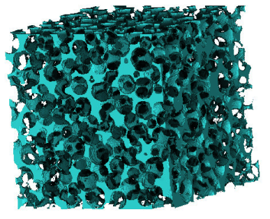
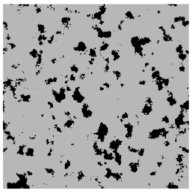
[220.6.1] The parameters for modeling the Fontainebleau sandstone
were 0.1 for the compaction factor, and
γ=-0.6 and b=2.9157 for the cementation parameters.
[220.6.2] The resulting model configuration of the sample DM is
displayed in Figure 2.
4.3 Gaussian Field Reconstruction Model
[222.1.1] A stochastic reconstruction model attempts to
approximate a given experimental sample by a randomly
generated model structure that matches prescribed
stochastic properties of the experimental sample.
[222.1.2] In this and the next section the stochastic property
of interest is the correlation function GEXr of
the Fontainebleau sandstone.
[222.2.1] The Gaussian field (GF) reconstruction model
tries to match a reference correlation function by
filtering Gaussian random variables [49, 2, 1, 69].
[222.2.2] Given the reference correlation function GEXr and
porosity ϕSEX of the experimental sample
the Gaussian field method proceeds in three main steps:
Initially a Gaussian field Xr is generated consisting of
statistically independent Gaussian random variables X∈R at each
lattice point r.
[222.2.3] The field Xr is first passed through a linear filter
which produces a correlated Gaussian field Yr with
zero mean and unit variance.
[222.2.4] The reference correlation function GEXr and porosity
ϕSEX enter into the mathematical construction
of this linear filter.
[222.2.5] The correlated field Yr is then passed through a nonlinear
discretization filter which produces the reconstructed sample SGF.
[222.2.6] Step 4.3 is costly
because it requires the solution of a very large set of
non-linear equations.
[222.2.7] A computationally more efficient
method uses Fourier Transformation [1].
[222.2.8] The linear filter in step 4.3
is defined in Fourier space through
where M=M1=M2=M3 is the sidelength of a cubic sample,
α=Md2 is a normalisation factor, and
| Xk=1Md∑rXre2πik⋅r | | (61) |
denotes the Fourier transform of Xr.
[222.2.9] Similarly Yk is the Fourier transform of Yr,
and GYk is the Fourier transform of the correlation
function GYr.
[222.2.10] GYr has to be computed by an
inverse process from the correlation function
GEXr and porosity of the experimental reference
(details in [1]).
[222.3.1] The Gaussian field reconstruction requires a large separation
ξEX≪N1/d where ξEX is the
correlation length of the experimental reference, and N=M1M2M3
is the number of sites.
[222.3.2] ξEX is defined as the length such that
GEXr≈0 for r>ξEX.
[222.3.3] If the condition ξEX≪N1/d is violated then step 4.3
of the reconstruction fails in the sense that the correlated
Gaussian field Yr does not have zero mean and unit variance.
[222.3.4] In such a situation the filter GYk will differ from the
Fourier transform of the correlation function of the Yr.
[222.3.5] It is also difficult to calculate GYr accurately near r=0
[1].
[222.3.6] This leads to a discrepancy at small r between GGFr and
GEXr.
[222.3.7] The problem can be overcome by choosing large M.
[222.3.8] However, in d=3 very large M also demands prohibitively
large memory.
[222.3.9] In
earlier work [2, 1] the correlation function
GEXr was sampled down to a lower resolution, and
the reconstruction algorithm then proceeded with such a
rescaled correlation function.
[224.0.1] This leads to a reconstructed sample SGF which
also has a lower resolution.
[224.0.2] Such reconstructions have lower average connectivity
compared to the original model [9]
For a quantitative comparison with the
microstructure of SEX it is necessary to retain the
original level of resolution,
and to use the original correlation
function GEXr without subsampling.
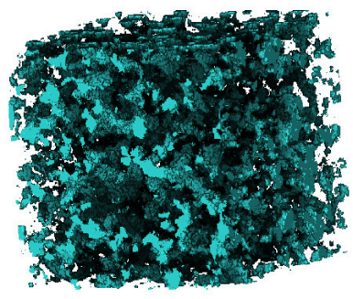
[224.0.3] Because GEXr is nearly 0 for r>30a
GEXr was truncated at r=30a to save computer time.
[224.0.4] The resulting configuration SGF with M=256
is displayed in Figure 3.
4.4 Simulated Annealing Reconstruction Model
[224.0.5] The simulated annealing (SA) reconstruction model is a
second method to generate a threedimensional random microstructure
with prescribed porosity and correlation function.
[224.0.6] The method generates a configuration SSA by minimizing
the deviations between GSAr and a predefined reference
function G0r.
[224.0.7] Note that the generated configuration
SSA is not unique and hence other modeling aspects
come into play [42].
[224.0.8] Below, G0r=GEXr is again the correlation function
of the Fontainebleau sandstone.
[224.1.1] An advantage of the simulated annealing method over the
Gaussian field method is that it can also be used to match other
quantities besides the correlation function.
[224.1.2] Examples would be the linear or spherical contact
distributions [42].
[224.1.3] On the other hand the method is computationally very demanding,
and cannot be implemented fully at present.
[224.1.4] A simplified implementation was discussed
in [70], and is used below.
[224.2.1] The reconstruction is performed on a cubic lattice with side length
M=M1=M2=M3 and lattice spacing a.
[224.2.2] The lattice is initialized randomly with 0’s and 1’s such that
the volume fraction of 0’s equals ϕSEX.
[224.2.3] This porosity is preserved throughout the simulation.
[224.2.4] For the sake of numerical efficiency the autocorrelation
function is evaluated in a simplified form using [70]
| | G~SArG~SA0-G~SA02+G~SA02= | |
| | =13M3∑rχMrχMr+re1+χMr+re2+χMr+re3 | | (62) |
where ei are the unit vectors in direction of the
coordinate axes, r=0,…,M2-1,
and where a tilde ~ is used to indicate the
directional restriction.
[224.2.5] The sum ∑r runs over all M3 lattice sites r
with periodic boundary conditions, i.e. ri+r is evaluated modulo M.
[224.3.1] A simulated annealing algorithm is used to minimize
the "energy" function
defined as the sum of the squared deviations of G~SA from the
experimental correlation function GEX.
[224.3.2] Each update starts with the exchange of two pixels, one
[page 226, §0]
from pore
space, one from matrix space.
[226.0.1] Let n denote the number of the proposed update step.
[226.0.2] Introducing an acceptance parameter Tn, which may be interpreted as an
n-dependent temperature, the proposed configuration is accepted with
probability
| p=min1,exp-En-En-1TnEn-1. | | (64) |
[226.0.3] Here the energy and the correlation function of the
configuration is denoted as En and G~SA,n, respectively.
[226.0.4] If the proposed move is rejected, then the old configuration is restored.
[226.1.1] A configuration with correlation GEX is found by lowering T.
[226.1.2] At low T the system approaches a configuration that minimizes
the energy function.
[226.1.3] In the simulations Tn was lowered with n as
[226.1.4] The simulation was stopped when 20000 consecutive updates were rejected.
[226.1.5] This happened after
2.5×10⁸
updates
(≈15 steps per site).
[226.1.6] The resulting configuration SSA for the simulated annealing
reconstruction is displayed in Figure 4.
[226.2.1] A complete evaluation of the correlation function as
defined in (29) for a threedimensional
system requires so much computer time, that it cannot
be carried out at present.
[226.2.2] Therefore the algorithm was simplified to increase its speed
[70].
[226.2.3] In the simplified algorithm the correlation function is only
evaluated along the
directions of the coordinate axes as indicated in (62).
[226.2.4] The original motivation was that for isotropic systems all
directions should be equivalent [70].
[226.2.5] However, it was found in [41] that as a result of
this simplification the reconstructed sample may
become anisotropic.
[226.2.6] In the simplified algorithm the correlation function of
the reconstruction deviates
from the reference correlation function in all directions other than
those of the axes [41].
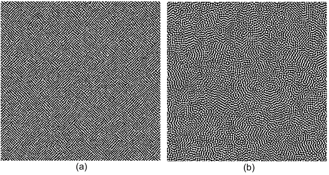
[226.2.7] The problem is illustrated in Figures 5(a) and
5(b) in two dimensions for a
reference correlation function given as
[226.2.8] In Figure 5(a) the correlation function was
matched only in the direction of the x- and y-axis.
[226.2.9] In Figure 5(b) the correlation function was
matched also along the diagonal directions obtained by
rotating the axes 45 degrees.
[226.2.10] The differences in isotropy of the two reconstructions
are clearly visible.
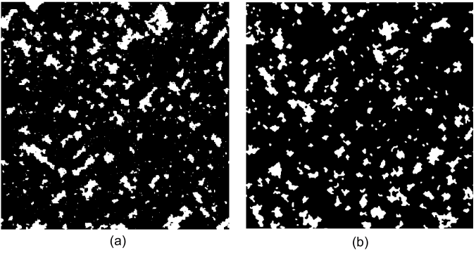
[226.2.11] In the special case of the correlation function of the
Fontainebleau sandstone, however, this effect seems to be
smaller.
[226.2.12] The Fontainebleau correlation function is given in Figure 7
below.
[226.2.13] Figure 6(a) and 6(b) show the result
of twodimensional reconstructions along the axes only
and along axes plus diagonal directions.
[226.2.14] The differences in isotropy seem to be less
pronounced.
[226.2.15] Perhaps this is due to the fact that the Fontainebleau
correlation function has no maxima and minima.