Article
[page 1, §1]
[1.1.1.1] Amorphous polymers and supercooled liquids
near the glass transition temperature are well known to
exhibit nonexponential relaxation behaviour in
many experiments [1].
[1.1.1.2] Dielectric spectroscopy, viscoelastic modulus measurements,
quasielastic light scattering, shear modulus and shear
compliance as well as specific heat measurements
all show strong deviations from the exponential Debye relaxation
function ![]() where
where ![]() is the relaxation time
[2].
is the relaxation time
[2].
[1.1.2.1] Most experimental works on glassy dynamics utilize only a small number of empirical nonexponential expressions when fitting to the observed experimental relaxation data. [1.1.2.2] All of these phenomenological fitting formulae are obtained by the method of introducing a fractional “stretching” exponent into the Debye expression in the time or frequency domain. [1.1.2.3] In the time domain this method leads to the “stretched exponential” or Kohlrausch relaxation function given as
| (1) |
with exponent ![]() and time constant
and time constant
![]() [3].[1.1.2.4] Of course all formulae obtained by the method of stretching
exponents are constructed such that they reduce to the
exponential Debye expression when
the stretching exponent becomes unity.
[1.1.2.5] Relaxation in the frequency domain is described
in terms of a normalized complex susceptibility
[3].[1.1.2.4] Of course all formulae obtained by the method of stretching
exponents are constructed such that they reduce to the
exponential Debye expression when
the stretching exponent becomes unity.
[1.1.2.5] Relaxation in the frequency domain is described
in terms of a normalized complex susceptibility
| (2) |
where ![]() ,
, ![]() is the frequency,
is the frequency,
![]() is a dynamic susceptibility normalized
by the corresponding isothermal susceptibility,
is a dynamic susceptibility normalized
by the corresponding isothermal susceptibility,
![]() is the static
susceptibility,
is the static
susceptibility,
![]() gives the “instantaneous” response,
and
gives the “instantaneous” response,
and ![]() is the Laplace transform of the
relaxation function
is the Laplace transform of the
relaxation function ![]() .
[1.1.2.6] Extending the method of stretching exponents to
the frequency domain one obtains
the Cole-Cole susceptibility [4]
.
[1.1.2.6] Extending the method of stretching exponents to
the frequency domain one obtains
the Cole-Cole susceptibility [4]
| (3) |
the Davidson-Cole expression [5]
| (4) |
or the combined Havriliak-Negami form [6] given in eq. (22) below. [1.2.0.1] Most surprisingly, the analytical transformations between the time and frequency domain for general values of the parameters in these simple analytical expressions seem to be unknown [7], and authors working in the time domain usually employ the stretched exponential function while authors working in the frequency domain use the stretched susceptibilities.
[1.2.1.1] Despite the fact that inserting the Kohlrausch function into equation (2) does not yield (3) or (4) (or the related Havriliak-Negami susceptibility in eq. (22) below) practitioners have tried to establish a relationship between these functions in order to facilitate the transition between the time and the frequency domain [7]. [1.2.1.2] Equally important for practical purposes is the transformation from expressions (3), (4) or (22) in the frequency domain to the corresponding relaxation functions in time [8]. [1.2.1.3] It seems therefore that analytical expressions for the Kohlrausch susceptibility in the frequency domain and for the Havriliak-Negami relaxation functions in the time domain are of general importance and broad interest.
[1.2.2.1] Great research activities have ensued from the observation
of Williams and Watts [3] that the Kohlrausch
susceptibility, obtained by inserting equation
(1) into equation (2),
has an analytical expression when ![]() .
Let me briefly recall their result.
[1.2.2.2] One defines the normalized relaxation function as
.
Let me briefly recall their result.
[1.2.2.2] One defines the normalized relaxation function as
| (5) |
where ![]() denotes an experimental relaxation
function (such as e.g. the electrical polarization
in dielectric experiments) normalized by the isothermal
susceptibility
denotes an experimental relaxation
function (such as e.g. the electrical polarization
in dielectric experiments) normalized by the isothermal
susceptibility ![]() .
[1.2.2.3] Recall now the well known Laplace transform [9]
.
[1.2.2.3] Recall now the well known Laplace transform [9]
| (6) |
[page 2, §0] where
| (7) |
denotes the complementary error function.
[2.1.0.1] Inserting this into equation (2) and restoring ![]() yields the known result[3]
yields the known result[3]
| (8) |
for the complex susceptibility.
[2.1.0.2] According to [7] there are no other cases
of ![]() for which an analytical expression
is known for the Kohlrausch susceptibility.
[2.1.0.3] My objectives in this paper are
(i) to provide analytical expressions
for the Kohlrausch susceptibility in the frequency
domain in terms of
for which an analytical expression
is known for the Kohlrausch susceptibility.
[2.1.0.3] My objectives in this paper are
(i) to provide analytical expressions
for the Kohlrausch susceptibility in the frequency
domain in terms of ![]() -functions for all
-functions for all ![]() ,
(ii) to derive analytical expressions
for the Davidson-Cole, Cole-Cole and Havriliak-Negami
relaxation functions in the time domain, and
(iii) to show that the approximate
correspondence between Kohlrausch and Havriliak-Negami
expressions in [7] is limited to a narrow frequency range.
,
(ii) to derive analytical expressions
for the Davidson-Cole, Cole-Cole and Havriliak-Negami
relaxation functions in the time domain, and
(iii) to show that the approximate
correspondence between Kohlrausch and Havriliak-Negami
expressions in [7] is limited to a narrow frequency range.
[2.1.1.1] The objectives of this paper are achieved by employing
a method based on so called ![]() -functions [10].
[2.1.1.2] The
-functions [10].
[2.1.1.2] The ![]() -function of order
-function of order ![]() and with parameters
and with parameters
![]() ,
, ![]() ,
,
![]() , and
, and ![]() is defined for
is defined for ![]() by the contour integral
[10, 11]
by the contour integral
[10, 11]
| (9) |
where the integrand is
 |
(10) |
In (9) ![]() and
and ![]() is not necessarily the principal value.
[2.1.1.3] The integers
is not necessarily the principal value.
[2.1.1.3] The integers ![]() must satisfy
must satisfy
| (11) |
and empty products are interpreted as being unity.
[2.1.1.4] For the conditions on the other parameters
and the path of integration the reader is referred
to the literature [10] (see [12, p. 120ff]
for a brief summary).
[2.1.1.5] The importance of these functions for the present purpose
arises from the facts that (i)
they contain most special
functions of mathematical physics as special cases
and (ii) their Laplace transform is again an ![]() -function.
[2.2.0.1] Moreover they possess series expansions that are
generalizations of hypergeometric series.
-function.
[2.2.0.1] Moreover they possess series expansions that are
generalizations of hypergeometric series.
[2.2.1.1] Based on the convenient properties of ![]() -functions
the first objective can now be tackled.
[2.2.1.2] An analytical expression for the Laplace transform of
the Kohlrausch function is obtained as
-functions
the first objective can now be tackled.
[2.2.1.2] An analytical expression for the Laplace transform of
the Kohlrausch function is obtained as
| (12) |
[2.2.1.3] The result is readily obtained from calculating formally
| (13) |
using the identification
| (14) |
and then employing identities among ![]() -functions [11, 12].
[2.2.1.4] Equation (12) answers the question raised in
Reference [7] concerning existence
of an analytical expression.
[2.2.1.5] It will be seen that
-functions [11, 12].
[2.2.1.4] Equation (12) answers the question raised in
Reference [7] concerning existence
of an analytical expression.
[2.2.1.5] It will be seen that ![]() -functions are
not more difficult to compute than other
transcendental functions.
[2.2.1.6] Inserting equation (12) into (2)
leads after some transformations involving
-functions are
not more difficult to compute than other
transcendental functions.
[2.2.1.6] Inserting equation (12) into (2)
leads after some transformations involving ![]() -function
identities to the Kohlrausch susceptibility in the
simple form
-function
identities to the Kohlrausch susceptibility in the
simple form
| (15) |
[2.2.1.7] This analytical result reduces the calculation of the Kohlrausch susceptibility to a Mellin-Barnes integral of the form (9).
[2.2.2.1] For practical purposes it is also of interest to
have series expansions for the analytical results.
[2.2.2.2] A Taylor series expansion can be obtained from
equation (9) using the calculus of residues.
[2.2.2.3] It reads for the ![]() -function
-function
| (16) |
[page 3, §0] for ![]() .
[3.1.0.1] Using this result the Kohlrausch susceptibility is
found to have the series expansion (for
.
[3.1.0.1] Using this result the Kohlrausch susceptibility is
found to have the series expansion (for ![]() )
)
| (17) |
which reduces its computation to elementary additions and multiplications. [3.1.0.2] The result agrees with a direct evaluation of the Laplace transform of the series expansion for the stretched exponential function. [3.1.0.3] Finally, the asymptotic expansion
| (18) |
holds for ![]() .
[3.1.0.4] It shows that the imaginary part increases linearly at low
frequencies similar to the Cole-Davidson susceptibility.
.
[3.1.0.4] It shows that the imaginary part increases linearly at low
frequencies similar to the Cole-Davidson susceptibility.
[3.1.1.1] Using the method of ![]() -functions sketched above allows
also to find analytical expressions for the relaxation
functions corresponding to stretched susceptibilities.
[3.1.1.2] The results are summarized in the two tables below.
Table 1 gives all relaxation functions,
their
-functions sketched above allows
also to find analytical expressions for the relaxation
functions corresponding to stretched susceptibilities.
[3.1.1.2] The results are summarized in the two tables below.
Table 1 gives all relaxation functions,
their ![]() -function representations and their power series
expansions, while Table 2 summarizes the
susceptibilities
in the frequency domain, their
-function representations and their power series
expansions, while Table 2 summarizes the
susceptibilities
in the frequency domain, their ![]() -function representations
and their power series expansions.
[3.2.0.1] In these tables the notation
-function representations
and their power series expansions.
[3.2.0.1] In these tables the notation
| (19) |
denotes the complementary incomplete Gamma function, and the abbreviation
| (20) |
is the Mittag-Leffler function. In addition the short hand notation
| (21) |
was introduced for writing the Kohlrausch susceptibility.
|
|
series | |||
|---|---|---|---|---|
| Debye | ![\begin{array}[]{c}\displaystyle\sum _{{k=0}}^{\infty}\frac{(-1)^{k}}{\Gamma(k+1)}\left(\frac{t}{{\tau}}\right)^{k}\\
\exp(-t/{\tau})\\
\end{array}](mi/mi60.png) |
![\begin{array}[]{r}\displaystyle\frac{t}{{\tau}}<\infty\\
\\
\displaystyle\frac{t}{{\tau}}\to\infty\end{array}](mi/mi65.png) |
||
| Kohlrausch | ![\begin{array}[]{c}\displaystyle\sum _{{k=0}}^{\infty}\frac{(-1)^{k}}{\Gamma(k+1)}\left(\frac{t}{{\tau _{{\beta}}}}\right)^{{{\beta}k}}\\
\exp(-(t/{\tau _{{\beta}}})^{{\beta}})\end{array}](mi/mi59.png) |
![\begin{array}[]{r}\displaystyle\frac{t}{{\tau _{{\beta}}}}<\infty\\
\\
\displaystyle\frac{t}{{\tau _{{\beta}}}}\to\infty\end{array}](mi/mi63.png) |
||
| Cole-Cole | ![\begin{array}[]{cr}\displaystyle\sum _{{k=0}}^{\infty}\frac{(-1)^{k}}{\Gamma({\alpha}k+1)}\left(\frac{t}{{\tau}}\right)^{{{\alpha}k}}\\
\displaystyle\sum _{{k=1}}^{\infty}\frac{(-1)^{{k+1}}}{\Gamma(1-{\alpha}k)}\left(\frac{t}{{\tau _{{\alpha}}}}\right)^{{-{\alpha}k}}\end{array}](mi/mi50.png) |
![\begin{array}[]{r}\displaystyle\frac{t}{{\tau _{{\alpha}}}}<\infty\\
\\
\displaystyle\frac{t}{{\tau _{{\alpha}}}}\to\infty\end{array}](mi/mi62.png) |
||
| Cole-Davidson | ![\begin{array}[]{c}\displaystyle 1-\frac{1}{\Gamma({\gamma})}\sum _{{k=0}}^{\infty}\frac{(-1)^{k}}{(k+{\gamma})\Gamma(k+1)}\left(\frac{t}{{\tau _{{\gamma}}}}\right)^{{k+{\gamma}}}\\
\displaystyle\frac{\exp(-t/{\tau _{{\gamma}}})}{\Gamma({\gamma})}\left(\frac{t}{{\tau _{{\gamma}}}}\right)^{{{\gamma}-1}}\left[1+\sum _{{k=0}}^{\infty}\prod _{{j=1}}^{k}({\gamma}-j)\left[\frac{t}{{\tau _{{\gamma}}}}\right]^{{-k}}\right]\end{array}](mi/mi53.png) |
![\begin{array}[]{r}\displaystyle\frac{t}{{\tau _{{\gamma}}}}<\infty\\
\\
\displaystyle\frac{t}{{\tau _{{\gamma}}}}\to\infty\end{array}](mi/mi64.png) |
||
| Havriliak-Negami | ![\begin{array}[]{c}1-\displaystyle\frac{1}{\Gamma({\gamma})}H^{{11}}_{{12}}\left(\left[\frac{t}{{\tau _{{H}}}}\right]^{{\alpha}}\left|\begin{array}[]{l}{(1,1)}\\
{({\gamma},1)(0,{\alpha})}\end{array}\right.\right)\\
{\alpha}\neq 1\end{array}](mi/mi51.png) |
![\begin{array}[]{c}\displaystyle 1-\frac{1}{\Gamma({\gamma})}\sum _{{k=0}}^{\infty}\frac{(-1)^{k}\Gamma(k+{\gamma})}{\Gamma({\alpha}k+{\alpha}{\gamma}+1)\Gamma(k+1)}\left[\frac{t}{{\tau _{{H}}}}\right]^{{{\alpha}(k+{\gamma})}}\\
\displaystyle\frac{1}{\Gamma({\gamma})}\sum _{{k=1}}^{\infty}\frac{(-1)^{{k+1}}\Gamma(k+{\gamma})}{\Gamma(1-{\alpha}k)\Gamma(k+1)}\left(\frac{t}{{\tau _{{H}}}}\right)^{{-{\alpha}k}}\end{array}](mi/mi52.png) |
![\begin{array}[]{r}\displaystyle\frac{t}{{\tau _{{H}}}}<\infty\\
\\
\displaystyle\frac{t}{{\tau _{{H}}}}\to\infty\end{array}](mi/mi61.png) |
|
|
series | |||
|---|---|---|---|---|
| Debye | ![\begin{array}[]{c}\displaystyle\sum _{{k=0}}^{\infty}(-1)^{k}(u{\tau})^{{-k-1}}\\
\displaystyle\sum _{{k=0}}^{\infty}(-1)^{k}(u{\tau})^{k}\\
\end{array}](mi/mi56.png) |
![\begin{array}[]{r}|u{\tau}|>1\\
\\
|u{\tau}|<1\end{array}](mi/mi70.png) |
||
| Kohlrausch | ![\begin{array}[]{c}\displaystyle 1-\sum _{{k=0}}^{\infty}\frac{(-1)^{k}\Gamma((k+1)/{\beta})}{{\beta}\Gamma(k+1)}(u{\tau _{{\beta}}})^{{k+1}}\\
\displaystyle 1-\sum _{{k=0}}^{\infty}\frac{(-1)^{k}\Gamma({\beta}k+1)}{\Gamma(k+1)}(u{\tau _{{\beta}}})^{{-{\beta}k}}\\
\end{array}](mi/mi54.png) |
![\begin{array}[]{r}|u{\tau _{{\beta}}}|\to 0\\
\\
|u{\tau _{{\beta}}}|>0\end{array}](mi/mi68.png) |
||
| Cole-Cole | ![\begin{array}[]{c}\displaystyle\sum _{{k=0}}^{\infty}(-1)^{k}(u{\tau _{{\alpha}}})^{{{\alpha}k}}\\
-\displaystyle\sum _{{k=0}}^{\infty}(-1)^{k}(u{\tau _{{\alpha}}})^{{-{\alpha}(k+1)}}\\
\end{array}](mi/mi55.png) |
![\begin{array}[]{r}|u{\tau _{{\alpha}}}|<1\\
\\
|u{\tau _{{\alpha}}}|>1\end{array}](mi/mi67.png) |
||
| ColeDavidson | ![\begin{array}[]{c}\displaystyle\sum _{{k=0}}^{\infty}\frac{(-1)^{k}\Gamma(k+{\gamma})}{\Gamma({\gamma})\Gamma(k+1)}(u{\tau _{{\gamma}}})^{k}\\
-\displaystyle\sum _{{k=0}}^{\infty}\frac{(-1)^{k}\Gamma(k+{\gamma})}{\Gamma({\gamma})\Gamma(k+1)}(u{\tau _{{\gamma}}})^{{-(k+{\gamma})}}\\
\end{array}](mi/mi58.png) |
![\begin{array}[]{r}|u{\tau _{{\gamma}}}|<1\\
\\
|u{\tau _{{\gamma}}}|>1\end{array}](mi/mi69.png) |
||
| Havriliak-Negami | ![\begin{array}[]{c}\displaystyle\sum _{{k=0}}^{\infty}\frac{(-1)^{k}\Gamma(k+{\gamma})}{\Gamma({\gamma})\Gamma(k+1)}(u{\tau _{{H}}})^{{{\alpha}k}}\\
-\displaystyle\sum _{{k=0}}^{\infty}\frac{(-1)^{k}\Gamma(k+{\gamma})}{\Gamma({\gamma})\Gamma(k+1)}(u{\tau _{{H}}})^{{-{\alpha}(k+{\gamma})}}\\
\end{array}](mi/mi57.png) |
![\begin{array}[]{r}|u{\tau _{{H}}}|<1\\
\\
|u{\tau _{{H}}}|>1\end{array}](mi/mi66.png) |
[page 4, §1][4.1.1.1] Having computable analytical expressions at hand for the Kohlrausch susceptibility it becomes possible to investigate the mappings between the Kohlrausch susceptibility and the Havriliak-Negami susceptibility [6]
| (22) |
that were postulated in Ref. [7].
[4.1.1.2] Table I and Figure 5 in Ref. [7] present fits
for the Kohlrausch susceptibility using the Havriliak-Negami
expression as fit function.
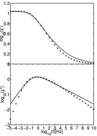
[4.1.1.3] Figure 1 shows real and imaginary part of
the Kohlrausch susceptibility with ![]() plotted
as crosses (
plotted
as crosses (![]() ) in a doubly logarithmic plot.
[4.1.1.4] The corresponding Havriliak-Negami fit from [7] with
) in a doubly logarithmic plot.
[4.1.1.4] The corresponding Havriliak-Negami fit from [7] with
![]() ,
, ![]() and
and ![]() is shown as the solid line. In all calculations
is shown as the solid line. In all calculations
![]() and
and ![]() unless stated otherwise.
unless stated otherwise.
[4.1.2.1] Because it is known that the phenomenological
susceptibility functions are often inadequate for
fitting experimental relaxation spectra, some researchers
prefer not to discuss stretching exponents but the
width of the imaginary part [13].
[4.1.2.2] Figure 2 plots three characteristic frequencies
for all three stretched susceptibility functions against
their respective
stretching exponent.
[4.2.0.1] The first is ![]() , the location of the maximum
of the imaginary part.
[4.2.0.2] The second is
, the location of the maximum
of the imaginary part.
[4.2.0.2] The second is ![]() , the location of the lower half
width point of the imaginary part.
[4.2.0.3] The third is
, the location of the lower half
width point of the imaginary part.
[4.2.0.3] The third is ![]() , the location of the upper half
width point of the imaginary part.
[4.2.0.4] The half width points are defined as the frequencies
at which the imaginary part has decayed to half of
its maximum value.
, the location of the upper half
width point of the imaginary part.
[4.2.0.4] The half width points are defined as the frequencies
at which the imaginary part has decayed to half of
its maximum value.
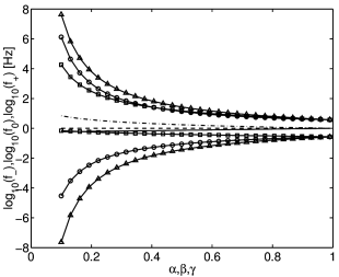
[4.2.1.1] Figure 2 shows that while the Cole-Cole
susceptibility (dashed line for maximum, solid line with
triangles for the half widths) is symmetric the other
two susceptibilities are asymmetric.
[4.2.1.2] For small values of ![]() resp.
resp. ![]() the
Cole-Davidson is more strongly asymmetric than the
Kohlrausch susceptibility.
[4.2.1.3] Note also that the lower halfwidth point moves to
higher frequencies for diminishing
the
Cole-Davidson is more strongly asymmetric than the
Kohlrausch susceptibility.
[4.2.1.3] Note also that the lower halfwidth point moves to
higher frequencies for diminishing ![]() in
the Cole-Davidson case.
[4.2.1.4] The total width of the relaxation peak in decades is
the difference between the upper and the lower half
width.
[4.2.1.5] For
in
the Cole-Davidson case.
[4.2.1.4] The total width of the relaxation peak in decades is
the difference between the upper and the lower half
width.
[4.2.1.5] For ![]() the total width of the Cole-Cole
function is roughly 7 decades, the width of the Kohlrausch
susceptibility is roughly 5 decades, and that of the
Cole-Davidson is roughly 2.5 decades.
[4.2.1.6] Figures 2 and 1
demonstrate that the mapping between
the Kohlrausch parameter
the total width of the Cole-Cole
function is roughly 7 decades, the width of the Kohlrausch
susceptibility is roughly 5 decades, and that of the
Cole-Davidson is roughly 2.5 decades.
[4.2.1.6] Figures 2 and 1
demonstrate that the mapping between
the Kohlrausch parameter ![]() and the Cole-Davidson
parameter
and the Cole-Davidson
parameter ![]() that is often employed by practitioners
[2] becomes increasingly inaccurate for small
values of the stretching exponents.
that is often employed by practitioners
[2] becomes increasingly inaccurate for small
values of the stretching exponents.
[page 5, §1][5.1.1.1] In summary the present paper has given unified representations
of nonexponential relaxation and non-Debye susceptibilities
in terms of ![]() -functions.
[5.1.1.2] These representations lead to computable expressions that
were used to investigate the relations between the
Kohlrausch susceptibility and other fit
functions.
[5.2.0.1] The
-functions.
[5.1.1.2] These representations lead to computable expressions that
were used to investigate the relations between the
Kohlrausch susceptibility and other fit
functions.
[5.2.0.1] The ![]() -function representations given here can help to
facilitate the computational transformation
between the frequency and time domain in
theoretical considerations and experiment.
-function representations given here can help to
facilitate the computational transformation
between the frequency and time domain in
theoretical considerations and experiment.
