4 Simulation Setup
[681.1.9.1] In this section we discuss how the experiment is represented mathematically.
[681.1.9.2] The four mass balance equations (1) are solved numerically.
[681.1.9.3] First, equations (6) and (7)
are used to eliminate S4 and P3.
[681.1.9.4] The primary variables are S1,S2,S3 and P1.
[681.1.9.5] The mass balances are discretized in space by cell centered finite volumes with upwind fluxes.
[681.1.9.6] They are discretized in time with a first order implicit fully coupled scheme.
[681.1.9.7] The corresponding system of nonlinear equations is solved with the Newton-Raphson method.
[681.1.9.8] The whole scheme is implemented in Matlab.
[681.1.9.9] The simulation is run with a resolution of one cell per centimeter,
i.e. with N=72 collocation points.
[681.1.9.10] Details of the algorithm are given elsewhere [3].
Table 1: List of parameters with units and their numerical values
used for simulating the experiment. Note that ϵM is a
mathematical regularization parameter, i.e. the limit ϵM→0
is implicit and it has been tested that the numberical results do not
change in this limit.
| Parameters |
Units |
Values |
| ϕ |
|
0.36 |
| ϵM |
|
0.01 |
| W |
O |
|
W |
O |
| ϱW |
ϱO |
kgm-3 |
1000 |
1.2 |
| SWdr |
SOim |
|
0.13 |
0.21 |
| η2 |
η4 |
|
6 |
4 |
| α |
β |
|
0.42 |
1.6 |
| Pa |
Pb |
Pa |
2700 |
3 |
| γ |
δ |
|
2.4 |
2.9 |
| P2* |
P4* |
Pa |
11000 |
3000 |
| R11 |
R33 |
kgm-3sec-1 |
3.83×10⁶ |
6.99×10⁴ |
| R22 |
R44 |
kgm-3sec-1 |
1016 |
1016 |
| Rij, i≠j |
kgm-3sec-1 |
0 |
[681.1.9.11] Dirichlet boundary conditions for the pressure P1 of the
percolating water phase are imposed at the lower boundary (x=0m),
where pressure is determined by the water reservoir.
[681.1.9.12] Dirichlet boundary conditions for the atmospheric pressure P3 of the percolating air
phase are chosen at the upper boundary (x=0.72m) of the column.
[681.1.9.13] All the other boundaries are impermeable so that the flux across them must vanish.
[681.1.9.14] The initial conditions are S1x,0=0.997,
S2x,0=0.001, S3x,0=0.001, S4x,0=0.001 for all
x∈0cm,72,cm
[681.1.9.15] Initial conditions for the pressures are not required because of the implicit formulation.
[681.1.9.16] Before the protocol for the pressure is started,
the system is given one day under hydrostatic
water pressure conditions to equilibrate.
[681.1.10.1] The parameters for the simulation are given in Table
1.
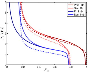
[681.1.10.2] They were obtained by fitting the primary drainage curve of the
capillary pressure saturation relationship obtained in
the residual decoupling approximation [9] to the
primary drainage curve of van Genuchten parametrization that
[15] obtained by a fit to data of the
first drainage process in the experiment.
[681.1.10.3] The van Genuchten parameters in [15]
are
αdr=4.28×10⁻⁴Pa-1, αim=8.56×10⁻⁴Pa-1,
ndr=5.52, nim=5.52, mdr=0.82, mim=0.82,
Swi=0.17, Snr=0.25.
[681.1.10.4] The resulting capillary pressure curves are compared in Figure 2.
[681.1.10.5] The viscous resistance coefficients were
obtained through R11≈μW/k, R33≈μO/k, where
k=33.7-12m2
was again taken from [15].
[681.1.10.6] The viscous resistance coefficients for the
non-percolating phases are assumed to be much larger than those
for the percolating phases R22,R44 ≫R11,R33.
[681.1.10.7] For the time-scale of the experiment
the results do not depend on the
numerical values of the resistance coefficients given in
Table 1 [3].