2.2 Mathematical Introduction to Fractional Derivatives
[22.1.1] The brief historical introduction has shown that fractional derivatives may be defined in numerous ways. [22.1.2] A natural and frequently used approach starts from repeated integration and extends it to fractional integrals. [22.1.3] Fractional derivatives are then defined either by continuation of fractional integrals to negative order (following Leibniz’ ideas [73]), or by integer order derivatives of fractional integrals (as suggested by Riemann [96]).
2.2.1 Fractional Integrals
2.2.1.1 Iterated Integrals
[22.2.1] Consider a locally integrable1 (This is a footnote:) 1
A function
[page 23, §0]
| (2.27) |
where
2.2.1.2 Riemann-Liouville Fractional Integrals
[23.1.1] Equation (2.27) for
| (2.28) |
is Euler’s
Definition 2.1
[23.2.1] Let
| (2.29) | ||
| for | ||
for
| (2.30) |
completes the definition.
[23.2.5] The definition may be generalized to
[page 24, §1]
[24.1.1] Formula (2.29a) appears in
[96, p.363] with
[24.2.1] The fractional integral operators
2.2.1.3 Weyl Fractional Integrals
[24.4.1] Examples (2.5) and (2.6) or
(A.3) and (A.5)
show that Definition 2.1 is well suited for
fractional integration of power series, but not for
functions defined by Fourier series.
[24.4.2] In fact, if
| (2.31) |
then the Riemann-Liouville fractional
[24.5.1] Functions on the unit circle
[page 25, §0]
| (2.32) |
with
| (2.33) |
for two periodic functions
Definition 2.2
[25.1.1] Let
| (2.34) |
where
| (2.35) |
for
[25.2.1] It can be shown that the series for
| (2.36) | ||
| respectively | ||
for
[page 26, §0]
fractional
integrals with limits
[26.1.1] The Weyl fractional integral may be rewritten as a convolution
| (2.37) |
where the convolution product for
functions on
| (2.38) |
and the convolution kernels are defined as
| (2.39) |
for
| (2.40) |
is the Heaviside unit step function,
and
| (2.41) |
is the Dirac
2.2.1.4 Riesz Fractional Integrals
[26.2.1] Riemann-Liouville and Weyl fractional integrals have upper or lower limits of integration, and are sometimes called left-sided resp. right-sided integrals. [26.2.2] A more symmetric definition was advanced in [97].
Definition 2.3
[26.3.1] Let
| (2.42) |
[page 27, §0] of right- and left-sided Weyl fractional integrals. [27.0.1] The conjugate Riesz potential is defined by
| (2.43) |
[27.0.2] Of course,
| (2.44) |
for
[27.1.1] Riesz fractional integration may be written as a convolution
| (2.45a) | |||
| (2.45b) |
with the (one-dimensional) Riesz kernels
| (2.46) |
for
| (2.47) |
for
| (2.48) |
with parameter
| (2.49) |
[27.1.4] This formula interpolates continuously from the Weyl integral
[page 28, §1]
2.2.1.5 Fractional Integrals of Distributions
[28.1.1] Fractional integration can be extended to distributions
using the convolution formula (2.37) above.
[28.1.2] Distributions are generalized functions [105, 31].
[28.1.3] They are defined as linear functionals on a space
| (2.50) |
where
| (2.51) |
for every test function
[28.2.1] In order to generalize (2.37) to distributions
one must define the convolution of two distributions.
[28.2.2] To do so one multiplies eq. (2.38) on both sides
with a smooth test function
| (2.52) |
where the notation
| (2.53) |
[page 29, §0]
where
Definition 2.4
[29.1.1] Let
| (2.54) |
for
[29.2.1] If
2.2.1.6 Integral Transforms
[29.3.1] The Fourier transformation is defined as
| (2.55) |
for functions
| (2.56) |
holds for
[29.4.1] For the Riesz potentials one has
| (2.57a) | |||
| (2.57b) |
for functions in Lizorkin space.
[page 30, §1] [30.1.1] The Laplace transform is defined as
| (2.58) |
for locally integrable functions
| (2.59) |
by the convolution theorem for Laplace transforms.
[30.1.3] The Laplace transform of
2.2.1.7 Fractional Integration by Parts
[30.2.1] If
| (2.60) |
holds.
[30.2.2] The formula is known as fractional integration by parts [99].
[30.2.3] For
| (2.61) |
holds for Weyl fractional integrals.
[30.3.1] These formulae provide a second method of generalizing fractional integration to distributions. [30.3.2] Equation (2.60) may be read as
| (2.62) |
for a distribution
2.2.1.8 Hardy-Littlewood Theorem
[30.4.1] The mapping properties of convolutions can be studied
with the help of Youngs inequality.
Let
[page 31, §0]
Theorem 2.5
[31.1.1] Let
2.2.1.9 Additivity
[31.2.1] The basic composition law for fractional integrals follows from
| (2.63) |
where Euler’s Beta-function
| (2.64) |
was used. [31.2.2] This implies the semigroup law for exponents
| (2.65) |
also called additivity law. [31.2.3] It holds for Riemann-Liouville, Weyl and Riesz-Feller fractional integrals of functions.
2.2.2 Fractional Derivatives
2.2.2.1 Riemann-Liouville Fractional Derivatives
[31.3.1] Riemann [96, p.341] suggested to define fractional derivatives as integer order derivatives of fractional integrals.
Definition 2.6
[31.4.1] Let
[page 32, §0]
functions such that
| (2.66) |
and
| (2.67) |
where5 (This is a footnote:) 5
[32.1.1] Here
[32.2.1] The notation for fractional derivatives is not
standardized6 (This is a footnote:) 6see footnote 2.1.
[32.2.2] Leibniz and Euler used
[32.3.1] Let
| (2.68) |
Substituting this into
| (2.69) |
where commutativity of
| (2.70) |
for
| (2.71) |
were used for the first order derivative.
[page 33, §1] [33.1.1] This observation suggests to introduce a modified Riemann-Liouville fractional derivative through
| (2.72) |
where
Theorem 2.7
[33.2.2] For
| (2.73) |
in terms of the Liouville(-Caputo) derivative defined in (2.72).
[33.3.1] The Riemann-Liouville fractional derivative is the left inverse of Riemann-Liouville fractional integrals. [33.3.2] More specifically, [99, p.44]
Theorem 2.8
[33.3.3] Let
| (2.74) |
holds for all
[33.4.1] For the right inverses of fractional integrals one finds
Theorem 2.9
[33.4.2] Let
| (2.75) |
holds.
[33.4.4] For
| (2.76) |
[33.5.1] The last theorem implies that for
| (2.77) |
[page 34, §0] holds only if
| (2.78) | ||
| and | ||
for all
2.2.2.2 General Types of Fractional Derivatives
[34.1.1] Riemann-Liouville fractional derivatives have been generalized in [52, p.433] to fractional derivatives of different types.
Definition 2.10
[34.2.1] The generalized Riemann-Liouville fractional derivative of order
| (2.79) |
for functions such that the expression on the right hand side exists.
[34.3.1] The type
2.2.2.3 Marchaud-Hadamard Fractional Derivatives
[34.4.1] Marchaud’s approach [78] is based on Hadamards finite parts of divergent integrals [36]. [34.4.2] The strategy is to define fractional derivatives as analytic continuation of fractional integrals to negative orders. [see [99, p.225]]
Definition 2.11
[34.5.1] Let
| (2.80) |
[page 35, §0]
and the
Marchaud fractional derivative of order
| (2.81) |
[35.0.1] For
| (2.82) |
[35.0.2] The definition is completed with
[35.1.1] The idea of Marchaud’s method is to extend
the Riemann-Liouville integral from
| (2.83) |
where
| (2.84) |
obtained by setting
| (2.85) |
[35.1.5] Formal integration by parts leads to
[35.2.1] The definition may be extended to
| (2.86) |
where
| (2.87) |
[page 36, §0]
is the translation operator.
[36.0.1] The Marchaud fractional derivative can then be
extended to
| (2.88) |
where
| (2.89) |
where the limit may be taken in the sense of pointwise or norm convergence.
[36.1.1] The Marchaud derivatives
[36.2.1] Let
2.2.2.4 Weyl Fractional Derivatives
[36.3.1] There are two kinds of Weyl fractional derivatives for periodic functions. [36.3.2] The Weyl-Liouville fractional derivative is defined as [99, p.351],[94]
| (2.90) |
for
| (2.91) |
for
| (2.92) |
coincides with the Riemann-Liouville derivative with
lower limit
[page 37, §1]
2.2.2.5 Riesz Fractional Derivatives
[37.1.1] To define the Riesz fractional derivative as integer derivatives of Riesz potentials consider the Fourier transforms
| (2.93) |
| (2.94) |
for
| (2.95) |
as a candidate for the Riesz fractional derivative.
[37.2.1] Following [94] the
strong Riesz fractional derivative of order
| (2.96) |
whenever it exists. [37.2.2] The convolution kernel defined as
| (2.97) |
is obtained from eq. (2.95).
[37.2.3] Indeed, this definition is equivalent to eq. (2.94).
[37.2.4] A function
2.2.2.6 Grünwald-Letnikov Fractional Derivatives
[37.3.1] The basic idea of the Grünwald approach is to generalize finite difference quotients to noninteger order, and then take the limit to obtain a differential quotient. [37.3.2] The first order derivative is the limit
| (2.98) |
of a difference quotient.
[37.3.3] In the last equality
| (2.99) |
is the translation operator.
[37.3.4] Repeated application of
| (2.100) |
[page 38, §0]
where
| (2.101) |
and the
| (2.102) |
which exhibits the similarity with the binomial formula.
[38.0.2] The generalization to noninteger
| (2.103) |
for
| (2.104) |
diverges as
| (2.105) |
Definition 2.12
[38.1.1] The Grünwald-Letnikov fractional derivative of order
| (2.106) |
of fractional difference quotients whenever the limit exists. [38.1.2] The Grünwald Letnikov fractional derivative is called pointwise or strong depending on whether the limit is taken pointwise or in the norm of a suitable Banach space.
[38.2.1] For a definition of Banach spaces and their norms see e.g. [128].
[38.3.1] The Grünwald-Letnikov fractional derivative
has been studied for periodic functions in
[page 39, §1]
Theorem 2.13
[39.1.1] Let
[39.1.3] There exists a function
[39.1.4] There exists a function
Theorem 2.14
[39.2.1] Let
2.2.2.7 Fractional Derivatives of Distributions
[39.3.1] The basic idea for defining fractional differentiation of
distributions is to extend the definition of fractional
integration (2.54) to negative
Definition 2.15
[39.4.1] Let
| (2.107) |
where
| (2.108) |
is the kernel distribution.
[39.4.3] For
| (2.109) |
where
[page 40, §1] [40.1.1] The kernel distribution in (2.108) is
| (2.110) |
for
| (2.111a) | |||
| (2.111b) | |||
| (2.111c) | |||
| (2.111d) |
where
| (2.112) |
then the Marchaud-Hadamard form is recovered with
[40.2.1] It is now possible to show that the convolution of distributions is in general not associative. [40.2.2] A counterexample is
| (2.113) |
where
[40.3.1]
Theorem 2.16
[40.3.3] If
| (2.114) |
with
[page 41, §1] [41.1.1] Note that
| (2.115) |
for all
| (2.116) |
holds for all
| (2.117) |
for all
2.2.2.8 Fractional Derivatives at Their Lower Limit
[41.3.1] All fractional derivatives defined above are nonlocal operators. [41.3.2] A local fractional derivative operator was introduced in [40, 41, 52].
Definition 2.17
[41.4.1] For
| (2.118) |
whenever the two limits exist and are equal.
[41.4.2] If
[41.5.1] These operators are useful for the analysis of singularities. [41.5.2] They were applied in [40, 41, 42, 44, 52] to the analysis of singularities in the theory of critical phenomena and to the generalization of Ehrenfests classification of phase transitions. [41.5.3] There is a close relationship to the theory of regularly varying functions [107] as evidenced by the following result [52].
Theorem 2.18
[41.6.1] Let the function
| (2.119) |
holds if and only if
| (2.120) |
holds.
[page 42, §1]
[42.1.1] A function
2.2.2.9 Fractional Powers of Operators
[42.2.1] The spectral decomposition of selfadjoint operators
is a familiar mathematical tool from quantum mechanics [116].
[42.2.2] Let
| (2.121) |
holds for all
| (2.122) |
on the domain
| (2.123) |
[42.2.6] Similarly, for any measurable
function
[42.3.1] Fractional powers of the Laplacian as the generator of the diffusion semigroup were introduced by Bochner [13] and Feller [26] based on Riesz’ fractional potentials. [42.3.2] The fractional diffusion equation
| (2.124) |
was related by Feller to the Levy stable laws [74] using
one dimensional fractional integrals
[page 43, §0]
semigroup
| (2.125) |
for every
2.2.2.10 Pseudodifferential Operators
[43.1.1] The calculus of pseudodifferential operators represents another generalization of the operator calculus in Hilbert spaces. [43.1.2] It has its roots in Hadamard’s ideas [36], Riesz potentials [97], Feller’s suggestion [26] and Calderon-Zygmund singular integrals [16]. [43.1.3] Later it was generalized and became a tool for treating elliptic partial differential operators with nonconstant coefficients.
Definition 2.19
[43.2.1] A (Kohn-Nirenberg) pseudodifferential operator of order
| (2.126) |
and the function
| (2.127) |
[43.2.3] The Hörmander symbol class
[43.3.1] Pseudodifferential operators provide a unified approach to differential and integral or convolution operators that are ‘‘nearly’’ translation invariant. [43.3.2] They have a close relation with Weyl quantization in physics [116, 28]. However, they will not be discussed further because the traditional symbol classes do not contain the usual fractional derivative operators. [43.3.3] Fractional Riesz derivatives are not pseudodifferential operators in the sense above. [43.3.4] Their symbols do not fall into any of the standard Kohn-Nirenberg or Hörmander symbol classes due to lack of differentiability at the origin.
[page 44, §1]
2.2.3 Eigenfunctions
[44.1.1] The eigenfunctions of Riemann-Liouville fractional derivatives are defined as the solutions of the fractional differential equation
| (2.128) |
where
| (2.129) |
where
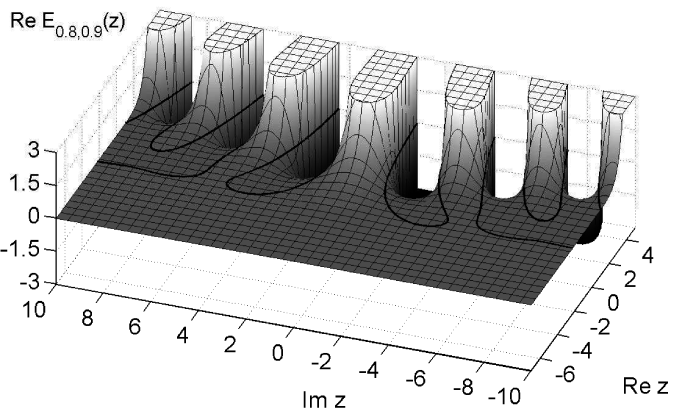
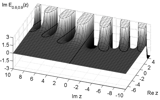
| (2.130) |
is the generalized Mittag-Leffler function [125, 126].
[44.1.3] More generally the eigenvalue equation for
fractional derivatives of order
| (2.131) |
and it is solved by [54, eq.124]
| (2.132) |
[page 45, §0]
where the case
| (2.133) |
with
| (2.134) |
where
[45.2.1] Note, that some authors are avoiding the operator
| (2.135) |
containing two derivative operators instead of one.
