[1286.4.1] Model A fits for 5-methyl-2-hexanol are shown in
Fig. 1 and for
methyl-m-toluate Fig. 2.
[1286.4.2] Note that in our notation ε=ε′-iε′′.
[1286.4.3] Model A fits the data remarkably well
for five, respectively seven orders of magnitude, where
both the α-peak and the excess wing can be fitted
simultaneously with only three parameters.
[1286.4.4] Model A is better suited than the Havriliak-Negami model which
only fits reasonably well for up to four orders of magnitudes
for these materials.
[1286.4.5] This improvement is due to the positive curvature
of the function in (11) at frequencies above
the α-peak.
[1286.4.6] Sometimes this curvature poses also the main difficulty
when fitting with model A.
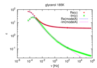
[1286.4.7] An example is glycerol as seen in the left part of Fig. 3.
[1286.4.8] While it is easy to fit closely the the α-peak
it is more difficult to simultaneously fit the excess wing.
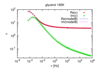
[1286.5.1] Model B can fit the data much better than model A, because
it contains one more parameter.
[1286.5.2] Nevertheless, it is remarkable that it can fit a range of up to 10 orders of
magnitude with little deviation from the data points.
[1286.5.3] We believe that this model can be used to fit over some more orders
of magnitude, but at this time there is no experimental data available
which covers a broader range.