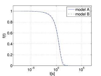
6 Representation of the solutions as functions of time
[1287.5.1] In [20]
we obtained the analytical solution of a fractional differential equation
of rational order, which we use to analyze our fitting results
for model A and model B.
[1287.5.2] For a general solution of equations (11) and (12)
with arbitrary real αi see [35].
[1287.5.3] The restriction to rational αi is not a drawback,
because we can approximate α1 and α2
by a rational value on a grid between 0 and 1.
[1287.5.4] This number of grid points is chosen to be 20, which keeps computation
times reasonably limited as the computing time increases quadratically
with the lowest common denominator of α with 1.
[page 1288, §1]
[1288.1.1] The solution for ft for model B is a sum
of Mittag-Leffler type functions:
| ft=∑j=1NBj∑k=0N-1cjN-k-1E-k/N,cjN;t, | | (14) |
where N is the smallest number for which both α1N and
α2N are integers.
[1288.1.2] The coefficients cj are the zeros of the characteristic polynomial
| cN+τ1α1cα1N+τ2α2cα2N+1=0, | | (15) |
the function Eν,a;t is defined as [36]
| Eν,a;t=tν∑k=0∞atkΓν+k+1. | | (16) |
[1288.1.3] The coefficients Bj are the solutions of
the linear system of equations
| ∑k=1NckiBk=0,0≤i≤N-α1N-1 | | | (17) |
| ∑k=1Ncki+τ1α1cki-N+α1NBk=0,N-α1N≤i≤N-α2N-1 | | | (18) |
| ∑k=1Ncki+τ1α1cki-N+α1N+τ2α2cki-N+α2NBk=0,N-α2N≤i≤N-2. | | | (19) |
[1288.1.4] This solution is only valid if all the roots cj
of the characteristic polynomial in (15)
are distinct, which is checked in the computations.
[1288.1.5] Because the linear system of equations (17)-(19) is
underdetermined we choose one fundamental solution for Bj and a
multiplication factor for ft such that f0=1.
[page 1289, §1]
[1289.1.1] The analytical solutions are plotted
for glycerol at 195K (Fig. 7).
[1289.1.2] The fitting values for τ for model A are τ1=4.991s
and τ2=1.089s.
[1289.1.3] Both values lie in the time interval where the relaxation occurs,
which confirms the interpretation of these fitting parameters as relaxation times.
[1289.1.4] For model B the fitted times are τ1=9.729s and τ2=0.92s.
[1289.1.5] So τ2 marks the onset of the relaxation and τ1 the end.
[1289.2.1] We note that the fractional derivatives appearing in
the initial value problem (7)
can be generalized to fractional derivatives
of arbitrary type β introduced in
[29]
and defined as
| Dfν,βt=ID1-βν-νIνfβν-νt,0≤β≤1. | | (20) |
[1289.2.2] For the case β=1 it reduces to the Riemann-Liouville
fractional derivative, while for β=0 to the
Liouville-Caputo-type derivative [33].
[1289.2.3] Because
| DEμ,a;tν,β=DEμ,a;tν,γ,0≤β,γ≤1,μ>-1,ν≥0, | | (21) |
the solution of our initial value problem does not change by replacing
the Riemann-Liouville fractional derivatives with these generalized
Riemann-Liouville fractional derivatives of type β.

