2 Definition of Models
[2.3.1] Consider first the integral equation of motion for the CTRW-model
[9, 10].
[2.3.2] The probability density pr,t obeys the
integral equation
| pr,t=δr0Φt+∫0tψt-t′∑r′λr-r′pr′,t′dt′ | | (3) |
where λr denotes the probability
for a displacement r in each single step, and ψt is the
waiting time distribution giving the probability density
for the time interval t between two consecutive steps.
[2.3.3] The transition probabilities obey ∑rλr=1,
and the function Φt is the survival probability at the initial
position which is related to the waiting time distribution through
[page 3, §0] Fourier-Laplace transformation leads to the
solution in Fourier-Laplace space given as [10]
| pk,u=1u1-ψu1-ψuλk | | (5) |
where pk,u is the Fourier-Laplace transform of
pr,t and similarly for ψ and λ.
[3.1.1] Two lattice models with different waiting time density will
be considered.
[3.1.2] In the first model
the waiting time density is chosen as the one found in
[1, 2]
| ψ1t=tα-1ταEα,α-tατα, | | (6) |
where 0<α≤1,0<τ<∞ is the characteristic time, and
| Ea,bx=∑k=0∞xkΓak+ba>0,b∈C. | | (7) |
is the generalized Mittag-Leffler function [14].
[3.1.3] In the second model
the waiting time density is chosen as
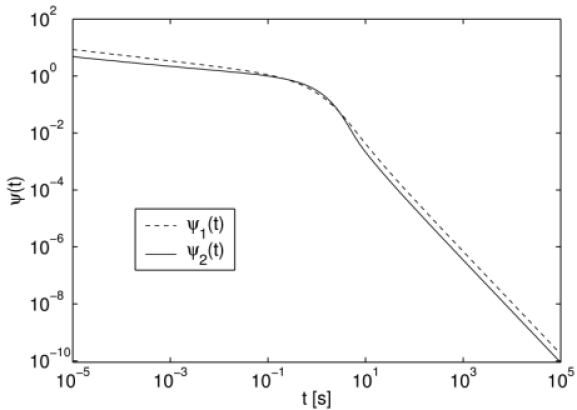
| ψ2t=tα-12cτ2Eα,α-tαcτ2+12τexp-t/τ | | (8) |
where 0<α≤1, 0<τ<∞ and c>0 is a suitable
dimensional constant.
[3.2.1] The waiting time density ψ2t differs only little
from ψ1t as shown graphically in Figure 1.
[3.2.2] Note that both models have a long time tail
of the form given in eq. (2), and
the average waiting time ∫0∞tψitdt diverges.
[3.3.1] For both models the spatial transition probabilities are
chosen as those for nearest-neighbour transitions (Polya walk)
on a d-dimensional hypercubic lattice given as
| λr=12d∑j=1dδr,-σej+δr,σej | | (9) |
where ej is the j-th unit basis vector generating the
lattice, σ>0 is the lattice constant and
δr,s=1 for r=s and
δr,s=0 for r≠s.