IV.A Examples
The present chapter begins the discussion of physical processes in porous media involving the transport or relaxation of physical quantities such as energy, momentum, mass or charge. As discussed in the introduction physical properties require equations of motion describing the underlying physical processes. Recurrent examples of experimental, theoretical and practical importance include :
-
the disordered diffusion equation
(4.1) where
 ,
,  is the thermal diffusivity tensor,
  is the space time
dependent temperature field,
is the space time
dependent temperature field,  is the density,
  the thermal conductivity and
  the specific heat at constant
pressure.
The superscript
the specific heat at constant
pressure.
The superscript  denotes transposition.
If the tensor field
denotes transposition.
If the tensor field  is sufficiently often differentiable
the equations are completed with boundary conditions at the sample
boundary
is sufficiently often differentiable
the equations are completed with boundary conditions at the sample
boundary  .
For the microscopic description of diffusion in a two component porous
medium
.
For the microscopic description of diffusion in a two component porous
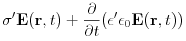
medium  whose components have diffusivities
 and
and  the diffusivity field has the
form
the diffusivity field has the
form ![{\bf D}({\bf r})={\bf D}_{\mathbb{P}}\chi\rule[-4.3pt]{0.0pt}{8.6pt}_{{\mathbb{P}}}({\bf r})+{\bf D}_{\mathbb{M}}\chi\rule[-4.3pt]{0.0pt}{8.6pt}_{{\mathbb{M}}}({\bf r})](mi/mi620.png) which is not differentiable at
which is not differentiable at  .
In such cases additional boundary conditions are required at the
internal interface , and the equation is interpreted
in the sense of distributions [259].
Typical values for sedimentary rocks are
.
In such cases additional boundary conditions are required at the
internal interface , and the equation is interpreted
in the sense of distributions [259].
Typical values for sedimentary rocks are
 Wm
Wm K,
K,
![\rho\rule[-4.3pt]{0.0pt}{8.6pt}_{{\mathbb{M}}}\approx 1..3](mi/mi607.png) g cm
g cm and
and  kJ kgK.
 -
the Laplace equation with variable coefficients
(4.2) where
 is again a second rank tensor field of local
transport coefficients,
is again a second rank tensor field of local
transport coefficients,  is a scalar field,
and the same remarks apply as for the diffusion equation
with respect to differentiability of and boundary
conditions.
For constant the equation reduces to the
Laplace equation
is a scalar field,
and the same remarks apply as for the diffusion equation
with respect to differentiability of and boundary
conditions.
For constant the equation reduces to the
Laplace equation  .
If the medium is random the coefficient matrix
.
If the medium is random the coefficient matrix  is a random function of
  .
Equation (4.2) is the basic
equation for the next chapter.
It is frequently obtained as the steady state limit
of the timedependent equations such as the diffusion
equation (4.1).
Other examples of (4.2) occur in
fluid flow, dielectric relaxation, or dispersion in
porous media.
In dielectric relaxation
.
Equation (4.2) is the basic
equation for the next chapter.
It is frequently obtained as the steady state limit
of the timedependent equations such as the diffusion
equation (4.1).
Other examples of (4.2) occur in
fluid flow, dielectric relaxation, or dispersion in
porous media.
In dielectric relaxation  is the electric potential
and is the matrix of local (spatially varying)
dielectric permittivity. In diffusion problems or heat
flow is the concentration field or temperature,
and the local diffusivity. In Darcy flow through
porous media is the pressure and is the
tensor of locally varying absolute permeabilities.
is the electric potential
and is the matrix of local (spatially varying)
dielectric permittivity. In diffusion problems or heat
flow is the concentration field or temperature,
and the local diffusivity. In Darcy flow through
porous media is the pressure and is the
tensor of locally varying absolute permeabilities.
-
the elastic wave equation is a system of equations for the three components
 of a vector displacement field
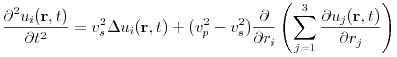
(4.3) where
 is the compressional and
  the shear wave
velocity of the material.
the shear wave
velocity of the material.
-
Maxwells equations in SI units for a medium with real dielectric constant
 , magnetic permeability
  and real
conductivity
and real
conductivity  and charge density
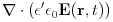


(4.4) 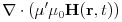

(4.5) 
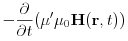
(4.6) 
(4.7) for the electric field
 , magnetic field
  supplemented by boundary conditions and the continuity equation
(4.8) Here
 F/m is the permittivity
and
F/m is the permittivity
and  H/m is the magnetic permeability
of empty space.
H/m is the magnetic permeability
of empty space. -
the Navier-Stokes equations for the velocity field
 and the pressure field
  of an incompressible liquid flowing through
the pore space
of an incompressible liquid flowing through
the pore space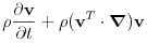
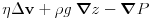
(4.9) 
(4.10) where
is the density and  the viscosity of the
liquid.
The coordinate system was chosen such that the acceleration
of gravity
the viscosity of the
liquid.
The coordinate system was chosen such that the acceleration
of gravity  points in the
  -direction.
These equations have to be supplemented with the no slip
boundary condition
-direction.
These equations have to be supplemented with the no slip
boundary condition  on the pore space boundary.
In the following mainly the equations for fluid transport and Maxwells equation for dielectric relaxation will be discussed in more detail. Combining fluid flow and diffusion into convection-diffusion equations yields the standard description for solute and contaminant transport [260, 261, 24, 262, 21, 26].
