8 Fitting the excess wing of glass-forming glycerol

[405.1.2.1] In this section the composite fractional susceptibility (of type $0<\mu<1$ ) given in eq. (36) is used to fit broad band dielectric data of glycerol [43, 20]. [405.1.2.2] For more discussion of the experimental data see the contribution of P. Lunkenheimer and A. Loidl in this special issue.

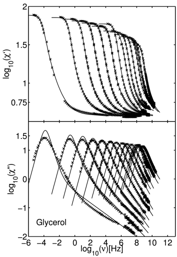
[405.1.3.1] Figure 1 shows a fit to the experimental data of glycerol with the composite fractional susceptibility function given in eq. (36). [405.1.3.2] The upper figure displays the real part, the lower figure the imaginary part of the frequency dependent susceptibility $\chi$ . [405.1.3.3] The different curves belong to different temperatures ranging from $T=323$ K down to $T=184K$ . [405.1.3.4] The normalized composite fractional susceptibility contains three fit parameters, while the traditionally used linear combination from eq. (27) contains six (resp. five when $\alpha _{2}=1$ ) fit parameters. [405.1.3.5] Because the experimental data are not normalized one additional parameter is needed in all cases to fit the data. [405.1.3.6] This extra paramter is the dielectric strength defined as

$\Delta\varepsilon=\chi(0)-\chi^{\infty}.$

(39)

[405.1.3.7] Figure 1 shows that not only the asymmetric $\alpha$ -peak but also the excess wing at high frequencies can be fitted quantitatively at all except the three lowest temperatures ( $T=204,195,184$ K) using the composite fractional susceptibility function (36) with only three essential fit parameters. [405.2.0.1] Note that for $T=213$ K the fit extends over almost 9 decades in frequency.

Figure 1: Separate fits for $\chi^{\prime}(\omega)$ (upper figure) and $\chi^{{\prime\prime}}(\omega)$ (lower figure) using the composite fractional susceptibility from eq. (36) for temperatures $T=$ 323, 303, 295, 289, 273, 263, 253, 243, 234, 223, 213, 204, 195, 184 K (from right to left) as function of frequency $\omega=2\pi\nu$ . The experimental data are taken from Ref. [43]. The corresponding fit parameters $\alpha,\tau _{1},\tau _{2}$ are shown in Figures 3 and 4. The dielectric strength $\Delta\varepsilon$ is plotted in Figure 3 as function of temperature.

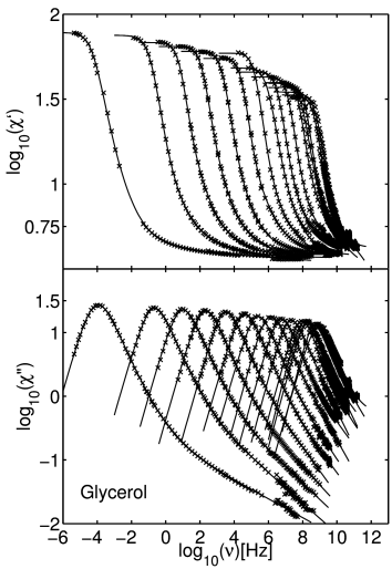
[405.2.1.1] If an iterated composite fractional time evolution [page 406, §0] with four parameters is introduced an even better quantitative agreement can be obtained at all availaible temperatures. [406.1.0.1] In Figure 2 the composite fractional susceptibility

$\hat{\chi}(u)=\frac{1+(\tau _{1}u)^{{\alpha _{1}}}+(\tau _{2}u)^{{\alpha _{2}}}}{1+\tau _{1}u+(\tau _{1}u)^{{\alpha _{1}}}+(\tau _{2}u)^{{\alpha _{2}}}}$

(40)

with four parameters was used to fit the same data as in Figure 1. [406.1.0.2] This fit function has still two (resp. one) parameter less than the conventional fit function of eq. (27). [406.1.0.3] Note that in this case for $T=184$ K the agreement extends over 13 decades in frequency including the full range of the excess wing.

Figure 2: Separate fits for $\chi^{\prime}(\omega)$ (upper figure) and $\chi^{{\prime\prime}}(\omega)$ (lower figure) using the composite fractional susceptibility from eq. (40) for temperatures $T=$ 323, 303, 295, 289, 273, 263, 253, 243, 234, 223, 213, 204, 195, 184 K (from right to left) as function of frequency $\omega=2\pi\nu$ . The experimental data the same as in Figure 1.

[406.1.1.1] The values of the fit parameters were found to depend sensitively on the frequency range that was included in the fit. [406.1.1.2] For this reason real and imaginary part were fitted separately. [406.1.1.3] The variation of the fit parameters for real and imaginary part gives an impression of the quality of the fit. [406.1.1.4] One source for parameter variations might be that the experimental data are patched together from differentmeasurements. [406.2.0.1] The matching of different data sets leads to visible breakpoints in the experimental data sets.

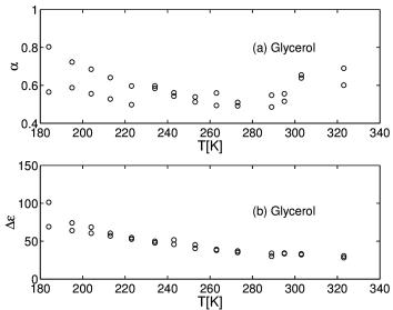
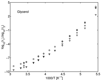
[406.2.1.1] In Figure 3 and 4 the fit parameters for real and imaginary parts corresponding to the fits shown in Figure 1 are plotted against temperature. [406.2.1.2] Figure 4 shows the relaxation times in an Arrhenius plot. [406.2.1.3] Clear deviations from Arrhenius behaviour are found. [406.2.1.4] Figure 3 shows the exponent $\alpha$ and dielectric strength $\Delta\varepsilon$ from the normalized composite fractional susceptibility. [page 407, §0] [407.1.0.1] Note that the dependence of $\alpha$ on temperature shows a qualitative different behaviour than for fits using Havriliak-Negami or Cole-Davidson functions. [407.1.0.2] In those cases the exponent decreases slowly with temperature from values around 0.8 to values around 0.5. [407.1.0.3] Here the values of $\alpha$ seem to remain flat for a temperature window between 200-300K where they fall into the range between $\alpha=0.5$ and $\alpha=0.6$ . [407.1.0.4] The values seem to increase with lowering the temperature, but this could be an artefact because the low temperature fits are only qualitatively accurate. [407.1.0.5] On the other hand the increase at low $T$ could also suggest a return to an effective non-fractional time evolution at low temperatures in the glassy phase. [407.1.0.6] For $\alpha\to 1$ the excess wing in the composite fractional susceptibility function becomes increasingly flat.

Figure 3: (a) Stretching exponent $\alpha$ from eq. (36) for the fits shown in Figure 1. (b) Dielectric strength $\Delta\varepsilon$ from eq. (39) for the fits based on eq. (36) shown in Figure 1. The two values at each temperature correspond to real and imaginary part $\chi^{{\prime}},\chi"$ .

Figure 4: Relaxation times $\tau _{1}$ (circles) and $\tau _{2}$ (triangles) from eq. (36) for the fits shown in Figure 1. The two values at each temperature correspond to real and imaginary part $\chi^{{\prime}},\chi^{{\prime\prime}}$ .

[407.1.1.1] In summary the present paper has derived a novel three parameter susceptibility function from the theory of fractional time evolutions [3]. [407.1.1.2] The new function contains only a single stretching exponent. [407.1.1.3] It shows two widespread characteristics of relaxation spectra in glass forming materials: i) an asymmetry of the $\alpha$ -peak and ii) an excess wing at high frequencies. [407.1.1.4] The excess wingis not shown by the popular Cole-Cole, Cole-Davidson, Havriliak-Negami or Kohlrausch-Williams-Watts functions. [407.1.1.5] The new fit function with only three parameters yields agreement with broad band dielectric data over up to 9 decades in time. [407.1.1.6] A four parameter generalization gives good agreement over up to 13 decades in frequency. [407.1.1.7] Nevertheless the large uncertainty in the fit parameters indicates that smoother experimental data are needed to establish conclusively whether composite fractional time evolutions exist in experiment.

Authors:	R. Hilfer und N.B. Wilding
originally published in:	Chemical Physics, Vol. 284, pages 399-408 (2002)
originally submitted:	December 7th, 2001