3 Saturation Overshoot
3.1 Experimental Observations
[2328.2.1] Infiltration experiments [59] on constant flux imbibition into a very dry porous medium report existence of non-monotone travelling wave profiles for the saturation [55, 62]
| (20) |
as a function of time ![]() and position
and position ![]() along the column.
[2328.2.2] Here
along the column.
[2328.2.2] Here ![]() denotes the similarity variable
denotes the similarity variable
| (21) |
and the parameter ![]() is the constant wave velocity.
[2328.2.3] From here on all quantitites
is the constant wave velocity.
[2328.2.3] From here on all quantitites ![]() are dimensionless.
[2328.2.4] The relation
are dimensionless.
[2328.2.4] The relation
| (22a) |
defines the dimensional depth coordinate ![]() increasing along the orientation of gravity.
[2328.2.5] The length
increasing along the orientation of gravity.
[2328.2.5] The length ![]() is the system size (length of column).
[2328.2.6] The dimensional time is
is the system size (length of column).
[2328.2.6] The dimensional time is
| (22b) |
where ![]() denotes the total (i.e. wetting plus nonwetting)
spatially constant flux through the column in m/s
(see eq. (13)).
[2328.2.7] The dimensional similarity variable reads
denotes the total (i.e. wetting plus nonwetting)
spatially constant flux through the column in m/s
(see eq. (13)).
[2328.2.7] The dimensional similarity variable reads
| (22c) |
[2328.2.8] Experimental observations show fluctuating profiles with an overshoot region [59, 73, 54, 55, 74, 75]. [2328.2.9] It can be viewed as a travelling wave profile consisting of an imbibition front followed by a drainage front.
3.2 Mathematical Formulation in d=1
[2328.3.1] The problem is to determine the height ![]() of the
overshoot region (=tip) and its velocity
of the
overshoot region (=tip) and its velocity ![]() given an initial profile
given an initial profile ![]() , the outlet saturation
, the outlet saturation ![]() ,
and the saturation
,
and the saturation ![]() at the
inlet as data of the problem.
[2328.3.2] Constant
at the
inlet as data of the problem.
[2328.3.2] Constant ![]() and constant
and constant ![]() are assumed for the
boundary conditions at the left boundary.
[2328.3.3] Note, that this differs from the experiment, where
the flux of the wetting phase and the pressure of the
nonwetting phase are controlled.
are assumed for the
boundary conditions at the left boundary.
[2328.3.3] Note, that this differs from the experiment, where
the flux of the wetting phase and the pressure of the
nonwetting phase are controlled.
[2328.4.1] The leading (imbibition) front is a solution of the nondimensionalized
fractional flow equation (obtained from eq. (17) for ![]() )
)
| (23a) | |
[page 2329, §0] while
| (23b) | |
must be fulfilled at the trailing (drainage) front.
[2329.0.1] Here ![]() is the porosity and the variables
is the porosity and the variables ![]() and
and ![]() have been nondimensionalized using the system size
have been nondimensionalized using the system size ![]() and the total flux
and the total flux ![]() . The latter is assumed to be constant.
[2329.0.2] The functions
. The latter is assumed to be constant.
[2329.0.2] The functions ![]() are the fractional flow
functions for primary imbibition and secondary drainage.
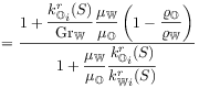
[2329.0.3] They are given as
are the fractional flow
functions for primary imbibition and secondary drainage.
[2329.0.3] They are given as
 |
(24a) | ||
 |
(24b) |
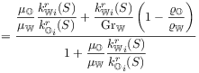
with ![]() and the dimensionless gravity number [76, 37]
and the dimensionless gravity number [76, 37]
| (25) |
defined in terms of total flux ![]() , wetting viscosity
, wetting viscosity ![]() ,
density
,
density ![]() , acceleration of gravity
, acceleration of gravity ![]() and absolute
permeability
and absolute
permeability ![]() of the medium.
[2329.0.4] The functions
of the medium.
[2329.0.4] The functions ![]() with
with ![]() are the relative permeabilities.
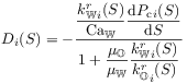
[2329.0.5] The capillary flux functions for drainage and imbibition
are defined as
are the relative permeabilities.
[2329.0.5] The capillary flux functions for drainage and imbibition
are defined as
 |
(26) |
with ![]() and a minus sign was introduced to make them positive.
[2329.0.6] The functions
and a minus sign was introduced to make them positive.
[2329.0.6] The functions ![]() are capillary pressure saturation
relations for drainage and imbibition.
[2329.0.7] The dimensionless number
are capillary pressure saturation
relations for drainage and imbibition.
[2329.0.7] The dimensionless number
| (27) |
is the macroscopic capillary number [76, 37]
with ![]() representing a typical (mean) capillary pressure
at
representing a typical (mean) capillary pressure
at ![]() (see eq. (34)).
[2329.0.8] For
(see eq. (34)).
[2329.0.8] For ![]() one has
one has ![]() and eqs. (23) reduce to two
nondimensionalized
Buckley-Leverett equations
and eqs. (23) reduce to two
nondimensionalized
Buckley-Leverett equations
| (28a) | |
for the leading (imbibition) front and
| (28b) | |
for the trailing (drainage) front.
[page 2330, §1]
3.3 Hysteresis
[2330.1.1] Conventional hysteresis models for the traditional theory require to store the process history for each location inside the sample [77, 78, 79]. [2330.1.2] Usually this means to store the pressure and saturation history (i.e. the reversal points, where the process switches between drainage and imbibition). [2330.1.3] A simple jump-type hysteresis model can be formulated locally in time based on eq. (23) as
| (29) |
[2330.1.4] Here ![]() denotes the left sided limit
denotes the left sided limit
| (30) |
![]() is the Heaviside step function (see eq. (35)),
and the parameter functions
is the Heaviside step function (see eq. (35)),
and the parameter functions ![]() with
with ![]() require
a pair of capillary pressure
and two pairs of relative permeability functions
as input.
[2330.1.5] The relative permeability functions employed for
computations are of van Genuchten form [80, 81]
require
a pair of capillary pressure
and two pairs of relative permeability functions
as input.
[2330.1.5] The relative permeability functions employed for
computations are of van Genuchten form [80, 81]
| (31a) | |||
| (31b) |
with ![]() and
and
| (32) |
the effective saturation. [2330.1.6] The resulting fractional flow functions with parameters from Table 1 are shown in Figure 1b. [2330.1.7] The capillary pressure functions used in the computations are
| (33) |
with ![]() and the typical pressure
and the typical pressure ![]() in (27)
is defined as
in (27)
is defined as
| (34) |
[2330.1.8] Equation (29) with initial and boundary
conditions for ![]() and an initial condition
for
and an initial condition
for ![]() is conjectured to be
a well defined semigroup of bounded operators on
is conjectured to be
a well defined semigroup of bounded operators on
![]() on a finite interval
on a finite interval ![]() of time.
[2330.1.9] The conjecture is supported by the fact that
each of the equations (23) individually
defines such a semigroup, and because multiplication by
of time.
[2330.1.9] The conjecture is supported by the fact that
each of the equations (23) individually
defines such a semigroup, and because multiplication by
![]() or
or ![]() are projection operators.
are projection operators.
