3 Averaged Induced Dynamics in the Ultralong Time Limit
[552.1.1]The induced transformations ![]() and
and ![]() were defined
for discrete time, and it is of interest to remove the discretization
to obtain the induced dynamics in continuous time.
[552.1.2]The conventional view on discrete vs. continuous time
in ergodic theory assumes
were defined
for discrete time, and it is of interest to remove the discretization
to obtain the induced dynamics in continuous time.
[552.1.2]The conventional view on discrete vs. continuous time
in ergodic theory assumes ![]() for the discretization time step, and holds that
“there is no essential difference between
discrete-time and continuous-time systems”[24],page 51.
1 (This is a footnote:) 1
It is argued that one
can always write
for the discretization time step, and holds that
“there is no essential difference between
discrete-time and continuous-time systems”[24],page 51.
1 (This is a footnote:) 1
It is argued that one
can always write ![]() as
as ![]() where
where
![]() is small and
is small and ![]() is the largest
integer not larger than
is the largest
integer not larger than ![]() . As long as
. As long as ![]() the continuous long time limit
the continuous long time limit ![]() corresponds
to the discrete long time limit
corresponds
to the discrete long time limit ![]() .
[552.1.3]Obviously, this equivalence between discrete and
continuous time breaks down for induced dynamics
because the continuous flow of time within
.
[552.1.3]Obviously, this equivalence between discrete and
continuous time breaks down for induced dynamics
because the continuous flow of time within ![]() is
interrupted by time periods of fluctuating length
during which the trajectory wanders outside
is
interrupted by time periods of fluctuating length
during which the trajectory wanders outside ![]() .
[552.1.4]These interruptions produce a discontinuous
(fluctuating) flow of time.
.
[552.1.4]These interruptions produce a discontinuous
(fluctuating) flow of time.
[552.2.1]There are three possibilities for removing the discretization
using a long time limit. [552.2.2]Only one of these employs the
conventional assumption ![]() (or
(or ![]() ). [552.2.3]The two
other alternatives are
). [552.2.3]The two
other alternatives are ![]() and
and ![]() . [552.2.4]The first alternative considers the limit
. [552.2.4]The first alternative considers the limit
![]() in which the discretization
step becomes small. [552.2.5]This possibility may be called the
short-long-time limit or continuous time limit,
and it was discussed in [21]. [552.2.6]The second alternative
is to consider the limit
in which the discretization
step becomes small. [552.2.5]This possibility may be called the
short-long-time limit or continuous time limit,
and it was discussed in [21]. [552.2.6]The second alternative
is to consider the limit ![]() in which the discretization step diverges
in which the discretization step diverges ![]() . [552.2.7]This
will be considered in this paper, and it is called the
long-long-time limit or the ultralong-time limit. [552.2.8]These limits are analogous to the ensemble limit
[18, 19, 20, 21].
. [552.2.7]This
will be considered in this paper, and it is called the
long-long-time limit or the ultralong-time limit. [552.2.8]These limits are analogous to the ensemble limit
[18, 19, 20, 21].
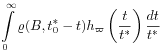
[552.3.1]According to its definition (8) the induced time
transformation ![]() acts as a convolution operator in time
acts as a convolution operator in time
| (9) |
[552.3.2]Applying the transformation ![]() times yields
times yields
| (10) |
[page 553, §0] where the last equation defines the ![]() -fold convolution
-fold convolution ![]() . [553.0.1]If
. [553.0.1]If ![]() exists this defines also
exists this defines also ![]() in the
in the ![]() long time limit.
long time limit.
[553.1.1]To determine whether a limiting density ![]() exists, note that
the
exists, note that
the ![]() -fold convolution
-fold convolution ![]() gives the probability
density
gives the probability
density ![]() Prob
Prob![]() of the random variable
of the random variable
![]() representing the sum of
representing the sum of ![]() independent and identically
distributed random recurrence times
independent and identically
distributed random recurrence times ![]() with common
lattice distribution
with common
lattice distribution ![]() . [553.1.2]A necessary and
sufficient condition for the existence of a limiting
density
. [553.1.2]A necessary and
sufficient condition for the existence of a limiting
density ![]() for suitably renormalized recurrence
times is that the discrete lattice probability density
for suitably renormalized recurrence
times is that the discrete lattice probability density
![]() belongs to the domain of attraction of a stable
density [25, 26]. [553.1.3]Then, because
belongs to the domain of attraction of a stable
density [25, 26]. [553.1.3]Then, because ![]() is defined as
the maximal value such that all the
is defined as
the maximal value such that all the ![]() are concentrated
on the arithmetic progression
are concentrated
on the arithmetic progression ![]() , it follows that for a
suitable choice of renormalization constants
, it follows that for a
suitable choice of renormalization constants ![]()
| (11) |
where ![]() is a limiting stable density
whose parameters obey
is a limiting stable density
whose parameters obey ![]() ,
, ![]() ,
,
![]() , and
, and ![]() [25, 26, 27]. [553.1.4]If
[25, 26, 27]. [553.1.4]If ![]() then the
limiting distribution is degenerate,
then the
limiting distribution is degenerate, ![]() for all values of
for all values of ![]() .
.
[553.2.1]The positivity of the recurrence times ![]() for all
for all
![]() implies that the renormalized recurrence times
implies that the renormalized recurrence times ![]() are bounded below, and this gives rise to the constraint
are bounded below, and this gives rise to the constraint
![]() for
for ![]() on the possible limiting distributions. [553.2.2]The limiting stable
distributions compatible with this constraint are given by
those with parameters
on the possible limiting distributions. [553.2.2]The limiting stable
distributions compatible with this constraint are given by
those with parameters ![]() and
and ![]() . [553.2.3]For
. [553.2.3]For ![]() the limiting densities may be abbreviated as
the limiting densities may be abbreviated as
| (12) |
which expresses the well known scaling relations for stable
distributions [25, 26, 18, 20]. [553.2.4]The scaling function ![]() can be expressed explicitly as
can be expressed explicitly as
| (13) |
in terms of general ![]() -functions whose definition may be found
in [28] or [18, 20]. [553.2.5]For
-functions whose definition may be found
in [28] or [18, 20]. [553.2.5]For ![]() one finds
one finds
| (14) |
the Dirac distribution concentrated at ![]() as the limiting
density. [553.2.6]If the limit exists and is nondegenerate,
i.e
as the limiting
density. [553.2.6]If the limit exists and is nondegenerate,
i.e ![]() , the renormalization constants
, the renormalization constants ![]() must have the form
must have the form
| (15) |
where ![]() is a slowly varying function [26], defined by
the condition that
is a slowly varying function [26], defined by
the condition that
| (16) |
for all ![]() .
.
[553.3.1]Using equations (11) and (12) one has for ![]()
| (17) |
[page 554, §0] where the centering constants have been chosen conveniently as ![]() . [554.0.1]From this it is clear that the traditional long time limit
. [554.0.1]From this it is clear that the traditional long time limit ![]() keeping
keeping ![]() finite produces
finite produces
![]() for
for ![]() finite, and thus
finite, and thus ![]() ,
unless
,
unless ![]() . [554.0.2]Therefore the conventional long time limit produces
a degenerate limiting distribution if it exists. [554.0.3]The ultralong
time limit on the other hand allows
. [554.0.2]Therefore the conventional long time limit produces
a degenerate limiting distribution if it exists. [554.0.3]The ultralong
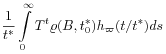
time limit on the other hand allows ![]() to become infinite. [554.0.4]If
to become infinite. [554.0.4]If ![]() diverges such that
diverges such that
| (18) |
exists, then this defines a renormalized ultralong continuous time,
![]() . [554.0.5]In this case
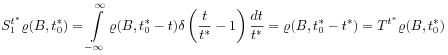
. [554.0.5]In this case ![]() contrary to the conventional limit. [554.0.6]It follows that
contrary to the conventional limit. [554.0.6]It follows that
![]() and thus from eq. (10) that
and thus from eq. (10) that
 |
(19) | |||
 |
where the ultralong time parameter ![]() was identified as
was identified as
| (20) |
[554.0.7]The identification of ![]() is justified for two reasons. [554.0.8]On the one hand
is justified for two reasons. [554.0.8]On the one hand
![]() for all
for all ![]() , where
, where ![]() is the expectation
with respect to the limiting distribution, and
is the expectation
with respect to the limiting distribution, and ![]() are two independent random recurrence times. [554.0.9]This shows that
are two independent random recurrence times. [554.0.9]This shows that
![]() has dimensions of time. [554.0.10]Secondly for
has dimensions of time. [554.0.10]Secondly for ![]() it
follows from (14) that
it
follows from (14) that
 |
(21) |
which again identifies ![]() as an ultralong time
parameter. [554.0.11]Note that the results (19) and (21)
imply macroscopic (=ultralong time) irreversibility by virtue
of (20) even if the underlying time evolution
as an ultralong time
parameter. [554.0.11]Note that the results (19) and (21)
imply macroscopic (=ultralong time) irreversibility by virtue
of (20) even if the underlying time evolution
![]() resp. [554.0.12]
resp. [554.0.12]![]() was reversible. [554.0.13]Perhaps this could provide
new insight into the longstanding irreversibility paradox. [554.0.14]The fundamental convolution semigroup (19) was first
obtained in [18, 19] and [21].
was reversible. [554.0.13]Perhaps this could provide
new insight into the longstanding irreversibility paradox. [554.0.14]The fundamental convolution semigroup (19) was first
obtained in [18, 19] and [21].
