IV Results
A Results for moments and cumulants
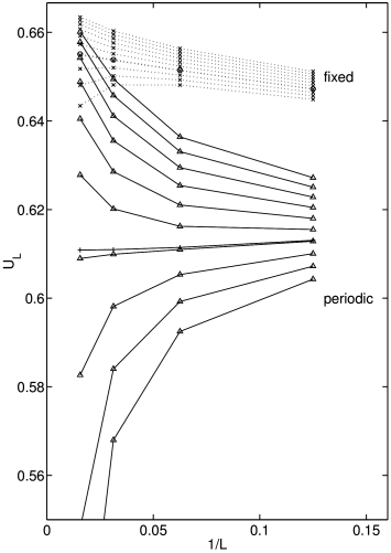
[71.1.3.1] In Figure 1 we compare the Binder cumulant for periodic and fixed boundary conditions.
[71.1.3.2] We notice that for fixed boundary conditions the values lie generally above those for the periodic case.
[71.1.3.3] They are very close to their upper limit ![]() , that is expected for a nonvanishing first moment.
, that is expected for a nonvanishing first moment.
B Results for maxima
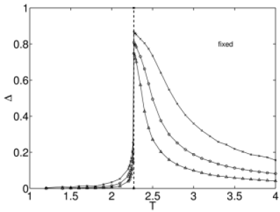
[71.1.4.1] For fixed boundary conditions the function ![]() has a single maximum
as a function of
has a single maximum
as a function of ![]() for all values of
for all values of ![]() and
and ![]() .
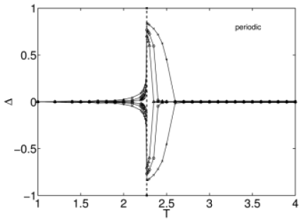
For periodic boundary conditions on the other hand there exists a temperature
.
For periodic boundary conditions on the other hand there exists a temperature ![]() above which the distribution has a single maximum, below which it has two local maxima.
[71.1.4.2] For
above which the distribution has a single maximum, below which it has two local maxima.
[71.1.4.2] For ![]() the most probable magnetization
approaches the exact infinite volume magnetization given by
the most probable magnetization
approaches the exact infinite volume magnetization given by
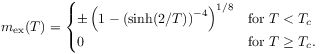 |
(18) |
[71.1.4.3] Therefore we utilize the difference
| (19) |
as a measure for the convergence to the infinite volume result.
[71.1.4.4] Here ![]() is the most probable magnetization defined earlier.
is the most probable magnetization defined earlier.
[71.1.5.1] In Figure 2 we plot this difference as a function of
temperature for system sizes ![]() for the case of fixed boundary conditions.
[71.1.5.2] One sees that for
for the case of fixed boundary conditions.
[71.1.5.2] One sees that for ![]() the difference is small.
[71.1.5.3] For
the difference is small.
[71.1.5.3] For ![]() the difference is rather large.
[71.1.5.4] This is surprising, as we shall see in more detail below.
[71.1.5.5] One also sees a pronounced maximum around
the difference is rather large.
[71.1.5.4] This is surprising, as we shall see in more detail below.
[71.1.5.5] One also sees a pronounced maximum around ![]() .
[71.1.5.6] The height of the maximum is so large that the results are clearly not
.
[71.1.5.6] The height of the maximum is so large that the results are clearly not ![]() -converged around
-converged around ![]() .
[71.1.5.7] The asymptotic
value for the maximum value at
.
[71.1.5.7] The asymptotic
value for the maximum value at ![]() is
is ![]() for all boundary conditions.
[71.2.0.1] There is no reason to believe that the shape of the critical order parameter distribution
has reached its asymptotic limit, if its peak (maximum value) has not reached its asymptotic limit.
for all boundary conditions.
[71.2.0.1] There is no reason to believe that the shape of the critical order parameter distribution
has reached its asymptotic limit, if its peak (maximum value) has not reached its asymptotic limit.
[71.2.1.1] In Figure 3 we plot ![]() for the case of periodic boundary conditions.
[71.2.1.2] In this case there are two local maxima below
for the case of periodic boundary conditions.
[71.2.1.2] In this case there are two local maxima below ![]() and in the critical region.
[71.2.1.3] Hence there are two curves.
[71.2.1.4] Compared to the case of fixed boundary conditions the deviations above
and in the critical region.
[71.2.1.3] Hence there are two curves.
[71.2.1.4] Compared to the case of fixed boundary conditions the deviations above ![]() appear to be smaller.
[71.2.1.5] A more detailed comparison to Gaussian behaviour, to be performed below, shows that
the deviations above
appear to be smaller.
[71.2.1.5] A more detailed comparison to Gaussian behaviour, to be performed below, shows that
the deviations above ![]() are comparable to those in the fixed case.
are comparable to those in the fixed case.
C Results for tails
[71.2.2.1] Here we analyze the tails of ![]() . First we find numbers
. First we find numbers ![]() such that the rescaled function
such that the rescaled function
| (20) |
where ![]() and
and ![]() has mean zero, unit norm and unit variance.
[71.2.2.2] To facilitate the comparison between periodic and fixed boundary conditions the data
for periodic boundary conditions were treated somewhat differently than it is normally done.
[71.2.2.3] In the periodic case eq. (20) is applied not to
has mean zero, unit norm and unit variance.
[71.2.2.2] To facilitate the comparison between periodic and fixed boundary conditions the data
for periodic boundary conditions were treated somewhat differently than it is normally done.
[71.2.2.3] In the periodic case eq. (20) is applied not to ![]() itself
but only to its right half, i.e. the data for
itself
but only to its right half, i.e. the data for ![]() .
In Figure 4 we show the rescaled functions
.
In Figure 4 we show the rescaled functions ![]() at
criticality
at
criticality ![]() for fixed and periodic boundary conditions.
[71.2.2.4] The data collapse at
for fixed and periodic boundary conditions.
[71.2.2.4] The data collapse at ![]() is found to be generally good.
is found to be generally good.
[71.2.3.1] To analyze the tails we split the function ![]() at the peak
into the left and right tail. More precisely we find the functions
at the peak
into the left and right tail. More precisely we find the functions
| (21) |
where ![]() is the position of the maximum.
[71.2.3.2] To exhibit stretched exponential tails we calculate the functions
is the position of the maximum.
[71.2.3.2] To exhibit stretched exponential tails we calculate the functions
| (22) |
where ![]() and plot them against
and plot them against ![]() .
[71.2.3.3] In this way of plotting the data a tail of the form
.
[71.2.3.3] In this way of plotting the data a tail of the form ![]() corresponds to the function
corresponds to the function
| (23) |
where ![]() and
and ![]() .
[71.2.3.4] The exponent
.
[71.2.3.4] The exponent ![]() can be easily identified as a plateau at the value
can be easily identified as a plateau at the value
![]() . In these plots the far tail regime corresponds to large values of
. In these plots the far tail regime corresponds to large values of ![]() .
[71.2.3.5] A standard normal (Gaussian) distribution
.
[71.2.3.5] A standard normal (Gaussian) distribution ![]() corresponds to the function
corresponds to the function
| (24) |
[page 72, §0]
where ![]() .
[72.1.0.1] We note that our choice to split
.
[72.1.0.1] We note that our choice to split ![]() at the peaks is natural, and we believe,
the only reasonable choice away from
at the peaks is natural, and we believe,
the only reasonable choice away from ![]() .
[72.1.0.2] At
.
[72.1.0.2] At ![]() , multiplication of algebraic prefactors or splitting the distribution differently
into right and left tails does not affect the results of the following analysis of the far tail region.
, multiplication of algebraic prefactors or splitting the distribution differently
into right and left tails does not affect the results of the following analysis of the far tail region.
[72.1.1.1] In the following we plot the results of our tail analysis
for three selected temperatures ![]() ,
, ![]() and
and ![]() .
[72.1.1.2] We have chosen these temperatures to demonstrate the degree of convergence
with respect to
.
[72.1.1.2] We have chosen these temperatures to demonstrate the degree of convergence
with respect to ![]() below
below ![]() , at
, at ![]() and above
and above ![]() .
[72.1.1.3] Below and above
.
[72.1.1.3] Below and above ![]() the central limit theorem predicts
Gaussian tails which would correspond to a plateau at 2 in our plots.
[72.1.1.4] At
the central limit theorem predicts
Gaussian tails which would correspond to a plateau at 2 in our plots.
[72.1.1.4] At ![]() theory predicts a right tail of the form
theory predicts a right tail of the form ![]() corresponding to a plateau at 16.
corresponding to a plateau at 16.
[72.1.2.1] In Figures 5-7 these are presented for three different temperatures. [72.1.2.2] Each of the three figures shows the left tail in the upper row and the right tail in the lower row of the figure. [72.1.2.3] Fixed boundary conditions appear in the left column, and periodic boundary conditions in the right column.
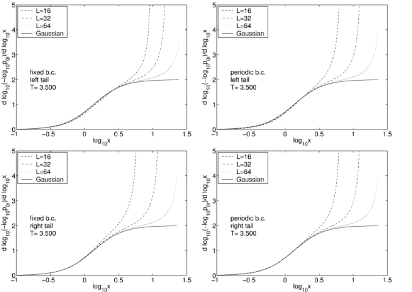
[72.1.3.1] All the plots in Figure 5 for the high temperature ![]() are similar.
[72.1.3.2] All tails approach the solid line from the top as
are similar.
[72.1.3.2] All tails approach the solid line from the top as ![]() is increased.
[72.1.3.3] The solid line represents a Gaussian distribution as expected from the central limit theorem.
[72.1.3.4] However, all the data, even those for
is increased.
[72.1.3.3] The solid line represents a Gaussian distribution as expected from the central limit theorem.
[72.1.3.4] However, all the data, even those for ![]() , match the Gaussian form over a relatively
narrow range in
, match the Gaussian form over a relatively
narrow range in ![]() .
[72.1.3.5] Note that this match still means agreement over many orders of magnitudes in the probability.
[72.1.3.6] In our analysis the plateau at 2 is beginning to become visible in the data.
[72.1.3.7] The emergence of the Gaussian tails
.
[72.1.3.5] Note that this match still means agreement over many orders of magnitudes in the probability.
[72.1.3.6] In our analysis the plateau at 2 is beginning to become visible in the data.
[72.1.3.7] The emergence of the Gaussian tails ![]() is slow, and
system sizes of at least
is slow, and
system sizes of at least ![]() are necessary to clearly show the plateau at 2.
are necessary to clearly show the plateau at 2.
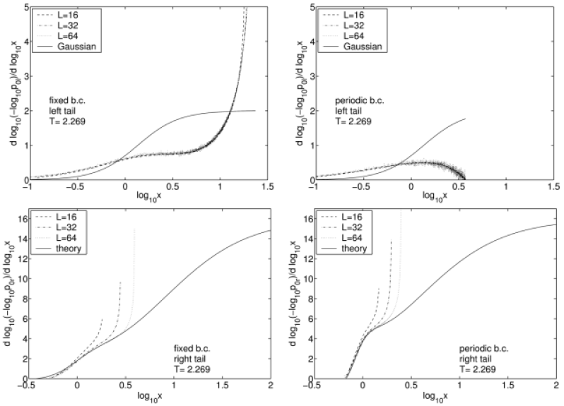
[72.1.4.1] Figure 6 shows the results for the tails of the critical order parameter distribution.
[72.1.4.2] The curves for the left tails (upper row) for all the three different system sizes nearly collapse.
[72.1.4.3] Deviations appear only at larger values of the scaling variable ![]() .
[72.1.4.4] The data collapse makes it difficult to see any systematic approach to
the limiting function for infinite systems.
[72.1.4.5] It should be kept in mind that the scaling function has not reached its form for infinite
systems, because the data collapse extends only over a narrow absolute range in the scaling variable
.
[72.1.4.4] The data collapse makes it difficult to see any systematic approach to
the limiting function for infinite systems.
[72.1.4.5] It should be kept in mind that the scaling function has not reached its form for infinite
systems, because the data collapse extends only over a narrow absolute range in the scaling variable ![]() .
[72.1.4.6] For fixed boundary conditions a plateau seems to
develop at around
.
[72.1.4.6] For fixed boundary conditions a plateau seems to
develop at around ![]() .
[72.1.4.7] It would correspond to an anomalous stretched exponential tail of the scaling function.
[72.1.4.8] To the best of our knowledge this has not been observed or predicted up to now.
.
[72.1.4.7] It would correspond to an anomalous stretched exponential tail of the scaling function.
[72.1.4.8] To the best of our knowledge this has not been observed or predicted up to now.
[72.1.5.1] Next we turn to the right tail of the order parameter distribution at ![]() .
[72.1.5.2] This tail is expected to behave as
.
[72.1.5.2] This tail is expected to behave as ![]() corresponding to a plateau
at 16 for large
corresponding to a plateau
at 16 for large ![]() [4, 3].
[72.1.5.3] Our data reveal a shoulder developing with increasing
[4, 3].
[72.1.5.3] Our data reveal a shoulder developing with increasing ![]() .
[72.1.5.4] We have fitted the right tail using this theoretical prediction.
[72.1.5.5] The fit is shown as a guide to the eye in Figure 6 using eq. (23)
with appropriate fit parameters.
[72.1.5.6] Because of the shift parameter
.
[72.1.5.4] We have fitted the right tail using this theoretical prediction.
[72.1.5.5] The fit is shown as a guide to the eye in Figure 6 using eq. (23)
with appropriate fit parameters.
[72.1.5.6] Because of the shift parameter ![]() in eq. (20) the predicted plateau at 16
appears for fully MCS-converged simulations at larger values of
in eq. (20) the predicted plateau at 16
appears for fully MCS-converged simulations at larger values of ![]() .
.
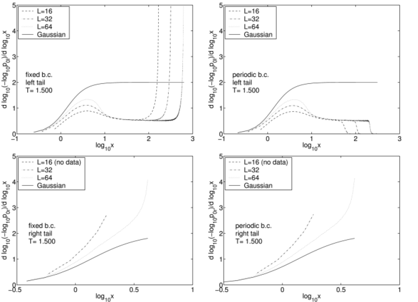
[72.1.6.1] Figure 7 for ![]() shows some important results.
[72.2.0.1] First consider the left tails in the upper row. Near the peak (i.e. for small
shows some important results.
[72.2.0.1] First consider the left tails in the upper row. Near the peak (i.e. for small ![]() ),
the curves approach Gaussian behaviour as one would expect from the central limit theorem [13].
[72.2.0.2] However, there is only a relatively narrow regime over which Gaussian behaviour is seen.
[72.2.0.3] In the intermediate range of
),
the curves approach Gaussian behaviour as one would expect from the central limit theorem [13].
[72.2.0.2] However, there is only a relatively narrow regime over which Gaussian behaviour is seen.
[72.2.0.3] In the intermediate range of ![]() the curves for the left tail show a plateau occuring at
the curves for the left tail show a plateau occuring at ![]() corresponding to a fat stretched exponential tail
corresponding to a fat stretched exponential tail ![]() .
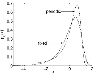
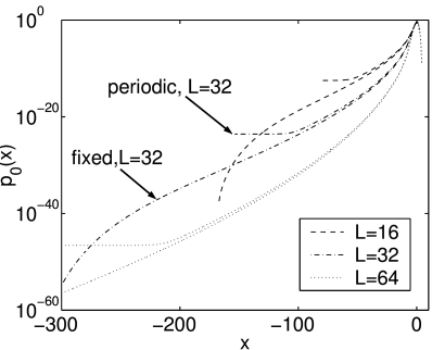
[72.2.0.4] In Figure 8 we show the full rescaled order parameter distributions at
.
[72.2.0.4] In Figure 8 we show the full rescaled order parameter distributions at ![]() .
[72.2.0.5] In the upper right hand corner of Figure 8 one sees a narrow Gaussian peak near
.
[72.2.0.5] In the upper right hand corner of Figure 8 one sees a narrow Gaussian peak near ![]() .
[72.2.0.6] It is followed by a stretched exponential tail.
[72.2.0.7] For periodic boundary conditions the stretched exponential tail crosses over into a flat bottom.
[72.2.0.8] For fixed boundary conditions the same stretched exponential tail is cutoff by a cutoff function.
[72.2.0.9] The stretched exponential tail represents the well known droplet regime
found analytically by Shlosman [29].
[72.2.0.10] We found this stretched exponential tail in the distributions for the low temperatures all the
way up to the critical temperature.
[72.2.0.11] Finally in the far tail regime the cutoff function lets
the curves diverge to infinity
for fixed boundary conditions.
[72.2.0.12] In the case of periodic boundary conditions the order parameter distribution
becomes a small constant corresponding to the value zero in our way of plotting the data.
[72.2.0.13] This is again a well known phenomenon [29], reflecting phase coexistence on finite
lattices governed by strip-like spin configurations.
.
[72.2.0.6] It is followed by a stretched exponential tail.
[72.2.0.7] For periodic boundary conditions the stretched exponential tail crosses over into a flat bottom.
[72.2.0.8] For fixed boundary conditions the same stretched exponential tail is cutoff by a cutoff function.
[72.2.0.9] The stretched exponential tail represents the well known droplet regime
found analytically by Shlosman [29].
[72.2.0.10] We found this stretched exponential tail in the distributions for the low temperatures all the
way up to the critical temperature.
[72.2.0.11] Finally in the far tail regime the cutoff function lets
the curves diverge to infinity
for fixed boundary conditions.
[72.2.0.12] In the case of periodic boundary conditions the order parameter distribution
becomes a small constant corresponding to the value zero in our way of plotting the data.
[72.2.0.13] This is again a well known phenomenon [29], reflecting phase coexistence on finite
lattices governed by strip-like spin configurations.
[72.2.1.1] Next we turn to the right tails at ![]() .
[72.2.1.2] Because the temperature is very low the magnetization is close to unity.
[72.2.1.3] Therefore a peak develops only for larger system sizes explaining the absence of data for
.
[72.2.1.2] Because the temperature is very low the magnetization is close to unity.
[72.2.1.3] Therefore a peak develops only for larger system sizes explaining the absence of data for ![]() .
[72.2.1.4] Even for
.
[72.2.1.4] Even for ![]() only five data points exist to the right of the peak,
and hence we can only conclude that the right tails
seem to approach Gaussian behaviour with increasing
only five data points exist to the right of the peak,
and hence we can only conclude that the right tails
seem to approach Gaussian behaviour with increasing ![]() .
.
D Convergence estimate
[72.2.2.1] Our results above show clearly that system sizes up to ![]() do not
allow to determine the order parameter distribution at criticality.
[72.2.2.2] Even away from criticality such system sizes are not sufficient to
estimate the true Gaussian behaviour of the tails that has to emergein an infinite system.
do not
allow to determine the order parameter distribution at criticality.
[72.2.2.2] Even away from criticality such system sizes are not sufficient to
estimate the true Gaussian behaviour of the tails that has to emergein an infinite system.
[72.2.3.1] It is therefore of interest to estimate the values of ![]() that would
suffice to obtain the true order parameter distribution at the
critical point. We discuss two ad hoc methods for such an
estimate.
that would
suffice to obtain the true order parameter distribution at the
critical point. We discuss two ad hoc methods for such an
estimate.
[72.2.4.1] In the first method we extrapolate the peaks in Figures 2 and 3,
and demand that ![]() be smaller than some small threshold, e.g.
be smaller than some small threshold, e.g. ![]() .
[72.2.4.2] In Figures 9 and 10 we show extrapolations of
.
[72.2.4.2] In Figures 9 and 10 we show extrapolations of
![]() based on power law and logarithmic fits.
[72.2.4.3] We were unable to fit the data to an exponential fit function.
based on power law and logarithmic fits.
[72.2.4.3] We were unable to fit the data to an exponential fit function.
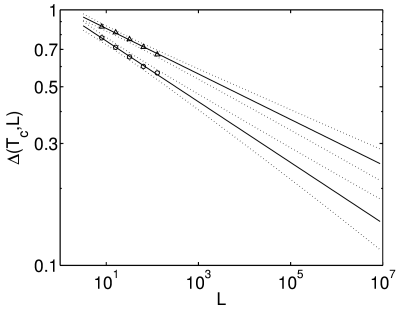
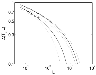
[72.2.5.1] We emphasize once more that the data points for ![]() are not MCS-converged and hence not fully reliable
[72.2.5.2] .
We also emphasize that the extrapolations are not meant to be accurate.
[72.2.5.3] Their only purpose is to provide
[page 73, §0]
an order of magnitude estimate for the values of
are not MCS-converged and hence not fully reliable
[72.2.5.2] .
We also emphasize that the extrapolations are not meant to be accurate.
[72.2.5.3] Their only purpose is to provide
[page 73, §0]
an order of magnitude estimate for the values of ![]() that we
believe are needed to find the true
that we
believe are needed to find the true ![]() -converged critical order parameter distribution.
[73.1.0.1] Extrapolations from both, periodic and fixed boundary conditions,
give values larger than
-converged critical order parameter distribution.
[73.1.0.1] Extrapolations from both, periodic and fixed boundary conditions,
give values larger than ![]() .
[73.1.0.2] Of course these values increase further
if one demands that the threshold value for
.
[73.1.0.2] Of course these values increase further
if one demands that the threshold value for ![]() is smaller than
is smaller than ![]() .
.
[73.1.1.1] A second method to estimate which values of ![]() are needed for the true
are needed for the true ![]() -converged form
of the critical order parameter distribution is to demand that the critical data collapse
should extend up to values of around 10 in the scaling variable
-converged form
of the critical order parameter distribution is to demand that the critical data collapse
should extend up to values of around 10 in the scaling variable ![]() .
[73.1.1.2] The range over which the data collapse determines the range over which the critical scaling function
can be considered to be known.
[73.1.1.3] From Figure 6 one sees that this range is only of the order
.
[73.1.1.2] The range over which the data collapse determines the range over which the critical scaling function
can be considered to be known.
[73.1.1.3] From Figure 6 one sees that this range is only of the order ![]() in our simulations.
[73.1.1.4] A range of
in our simulations.
[73.1.1.4] A range of ![]() might still be too small if one wants to decide
whether or not the distribution develops algebraic tails.
[73.1.1.5] Using a
value of
might still be too small if one wants to decide
whether or not the distribution develops algebraic tails.
[73.1.1.5] Using a
value of ![]() as a lower bound and remembering that
as a lower bound and remembering that ![]() one finds
one finds ![]() .
[73.2.0.1] Again this value is very high and in qualitative agreement with the high values
found from the first extrapolation method.
.
[73.2.0.1] Again this value is very high and in qualitative agreement with the high values
found from the first extrapolation method.
[73.2.1.1] Although we have analysed only periodic and fixed boundary conditions here,
some other boundary condition could be more relevant for such a study.
[73.2.1.2] At criticality, a fully converged distribution must correspond
to a value of ![]() close to zero.
[73.2.1.3] We find
close to zero.
[73.2.1.3] We find ![]() for periodic boundary condition to be smaller than
for periodic boundary condition to be smaller than
![]() for fixed boundary condition.
[73.2.1.4] So, perhaps, some other boundary condition may give the true critical order parameter
distribution at a lower value of
for fixed boundary condition.
[73.2.1.4] So, perhaps, some other boundary condition may give the true critical order parameter
distribution at a lower value of ![]() than the extrapolated system
sizes anticipated for these boundary conditions from the above analysis.
than the extrapolated system
sizes anticipated for these boundary conditions from the above analysis.
