3 Initial Conditions, Boundary Conditions and Model Parameters

[513.4.1] Consider a cylindrical column containing a homogeneous, isotropic and incompressible porous medium. [513.4.2] The column is closed at both ends and filled with two immiscible fluids. [513.4.3] Assume that the surface and interfacial tensions are such that the capillary fringe is much thicker than the column diameter so that a onedimensional description is appropriate.

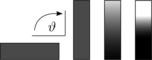
[513.5.1] The experimental situation considered here is that of raising a closed column as described in [26, p. 223]. [513.5.2] It is illustrated in Figure 1. [513.5.3] Initially, at instant $t=0$ , both fluids are at rest. [513.5.4] The column is oriented horizontally ( $\vartheta=0$ ), i.e., perpendicular to the direction of gravity. [513.5.5] The displacement processes are initiated by rotating the column into a vertical position. [513.5.6] The time protocol for rotating the column may generally be written as

$\vartheta(t)=\arcsin\left\{\frac{1}{2}\left[\tanh\left(\frac{t-t_{*}}{t_{{**}}}\right)+1\right]\right\}$

(14)

where $t_{*}$ is the instant of most rapid rotation and $t_{{**}}$ is the inverse rate of the rotation.

Figure 1: Raising a closed column according to the protocol of (14). Initially the column is oriented horizontally and the saturations are constant. Regions of high water saturation are indicated in darker shade, regions of high oil saturation are indicated in lighter shade. The last two columns illustrate the simultaneous imbibition (lower part of column) and drainage (upper part of column) processes that finally result in the formation of a capillary fringe.

[513.6.1] The constitutive equations yield the following system of $10$ coupled nonlinear partial differential equations

	$\displaystyle\quad\frac{\partial S_{1}}{\partial t}+\frac{\partial(S_{1}{v}_{1})}{\partial x}={\eta _{{2}}}\left(\frac{S_{2}-{{S_{2}}^{}}}{{{S_{{\mathbb{W}}}}^{}}-{S_{{\mathbb{W}}}}}\right)\frac{\partial{S_{{\mathbb{W}}}}}{\partial t}$		(15a)
	$\displaystyle\quad\frac{\partial S_{2}}{\partial t}+\frac{\partial(S_{2}{v}_{2})}{\partial x}=-{\eta _{{2}}}\left(\frac{S_{2}-{{S_{2}}^{}}}{{{S_{{\mathbb{W}}}}^{}}-{S_{{\mathbb{W}}}}}\right)\frac{\partial{S_{{\mathbb{W}}}}}{\partial t}$		(15b)
	$\displaystyle\quad\frac{\partial S_{3}}{\partial t}+\frac{\partial(S_{3}{v}_{3})}{\partial x}={\eta _{{4}}}\left(\frac{S_{4}-{{S_{4}}^{}}}{{{S_{{\mathbb{O}}}}^{}}-{S_{{\mathbb{O}}}}}\right)\frac{\partial{S_{{\mathbb{O}}}}}{\partial t}$		(15c)
	$\displaystyle\quad\frac{\partial S_{4}}{\partial t}+\frac{\partial(S_{4}{v}_{4})}{\partial x}=-{\eta _{{4}}}\left(\frac{S_{4}-{{S_{4}}^{}}}{{{S_{{\mathbb{O}}}}^{}}-{S_{{\mathbb{O}}}}}\right)\frac{\partial{S_{{\mathbb{O}}}}}{\partial t}$		(15d)
	$\displaystyle\varrho _{{\mathbb{W}}}\frac{{\rm D}^{1}}{{\rm D}t}{v}_{1}+\frac{\partial P_{1}}{\partial x}-\varrho _{{\mathbb{W}}}g\sin\vartheta$
	$\displaystyle\qquad=\sum _{{j=1}}^{{5}}\frac{R_{{1j}}}{\phi S_{1}}({v}_{j}-{v}_{1})-\frac{{\eta _{{2}}}{v}_{1}}{S_{1}}\left(\frac{S_{2}-{{S_{2}}^{}}}{{{S_{{\mathbb{W}}}}^{}}-{S_{{\mathbb{W}}}}}\right)\frac{\partial{S_{{\mathbb{W}}}}}{\partial t}$		(15e)
	$\displaystyle\varrho _{{\mathbb{W}}}\frac{{\rm D}^{2}}{{\rm D}t}{v}_{2}+\frac{\partial}{\partial x}(P_{3}-\gamma P^{*}_{2}S_{2}^{{\gamma-1}}-\Pi _{{\rm a}}S_{1}^{{-\alpha}})-\varrho _{{\mathbb{W}}}g\sin\vartheta$
	$\displaystyle\qquad=\sum _{{j=1}}^{{5}}\frac{R_{{2j}}}{\phi S_{2}}({v}_{j}-{v}_{2})+\frac{{\eta _{{2}}}{v}_{2}}{S_{2}}\left(\frac{S_{2}-{{S_{2}}^{}}}{{{S_{{\mathbb{W}}}}^{}}-{S_{{\mathbb{W}}}}}\right)\frac{\partial{S_{{\mathbb{W}}}}}{\partial t}$		(15f)
	$\displaystyle\varrho _{{\mathbb{O}}}\frac{{\rm D}^{3}}{{\rm D}t}{v}_{3}+\frac{\partial P_{3}}{\partial x}-\varrho _{{\mathbb{O}}}g\sin\vartheta$
	$\displaystyle\qquad=\sum _{{j=1}}^{{5}}\frac{R_{{3j}}}{\phi S_{3}}({v}_{j}-{v}_{3})-\frac{{\eta _{{4}}}{v}_{3}}{S_{3}}\left(\frac{S_{4}-{{S_{4}}^{}}}{{{S_{{\mathbb{O}}}}^{}}-{S_{{\mathbb{O}}}}}\right)\frac{\partial{S_{{\mathbb{O}}}}}{\partial t}$		(15g)
	$\displaystyle\varrho _{{\mathbb{O}}}\frac{{\rm D}^{4}}{{\rm D}t}{v}_{4}+\frac{\partial}{\partial x}(P_{1}-\delta P^{*}_{4}S_{4}^{{\delta-1}}-\Pi _{{\rm b}}S_{3}^{{-\beta}})-\varrho _{{\mathbb{O}}}g\sin\vartheta$
	$\displaystyle\qquad=\sum _{{j=1}}^{{5}}\frac{R_{{4j}}}{\phi S_{4}}({v}_{j}-{v}_{4})+\frac{{\eta _{{4}}}{v}_{4}}{S_{4}}\left(\frac{S_{4}-{{S_{4}}^{}}}{{{S_{{\mathbb{O}}}}^{}}-{S_{{\mathbb{O}}}}}\right)\frac{\partial{S_{{\mathbb{O}}}}}{\partial t}$		(15h)
	$\displaystyle\qquad S_{1}+S_{2}+S_{3}+S_{4}=1$		(15i)
	$\displaystyle\frac{\partial P_{3}}{\partial x}=\frac{\partial P_{1}}{\partial x}+\frac{\partial}{2\partial x}\left[\Pi _{{\rm a}}S_{1}^{{-\alpha}}-\Pi _{{\rm b}}S_{3}^{{-\beta}}+\gamma P^{}_{2}S_{2}^{{\gamma-1}}-\delta P^{}_{4}S_{4}^{{\delta-1}}\right]$		(15j)

[page 514, §0] where ${v}_{5}=0,R_{{12}}=0,R_{{34}}=0$ , and the quantities ${{S_{{\mathbb{W}}}}^{*}},{{S_{{\mathbb{O}}}}^{*}}$ , ${{S_{2}}^{*}},{{S_{4}}^{*}}$ are defined in eq. (7). [514.0.1] This system of $10$ equations is reduced to a system of only $9$ equations by inserting eq. (15j) into eqs. (15) and (15) to eliminate $\partial P_{3}/\partial x$ . [514.0.2] The remaining $9$ unknowns are $S_{i},{v}_{i},(i=1,2,3,4)$ and $P_{1}$ .

[514.1.1] The system (15) has to be solved subject to initial and boundary data. [514.1.2] No flow boundary conditions at both ends require

$\displaystyle{v}_{i}(0,t)$	$\displaystyle=0,\qquad i=1,2,3,4,$		(16a)
$\displaystyle{v}_{i}(L,t)$	$\displaystyle=0,\qquad i=1,2,3,4.$		(16b)

[514.1.3] The fluids are incompressible. [514.1.4] Hence the reference pressure can be fixed to zero at the left boundary

$P_{1}(0,t)=0.$

(17)

[514.1.5] The saturations remain free at the boundaries of the column.

[514.2.1] Initially the fluids are at rest and their velocities vanish. [514.2.2] The initial conditions are ( $i=1,2,3,4$ )

$\displaystyle{v}_{i}(x,0)$	$\displaystyle={v}_{i}^{0}(x)=0$	(18a)
$\displaystyle P_{1}$	$\displaystyle=P_{1}^{0}(x)=0$	(18b)
$\displaystyle S_{i}(x,0)$	$\displaystyle=S_{i}^{0}(x)=S_{i}^{0}.$	(18c)

[514.2.3] In the present study the initial saturations will be taken as constants, i.e. independent of $x$ .

[514.3.1] The model parameters are chosen largely identical to the parameters in [26]. [514.3.2] They describe experimental data obtained at the Versuchseinrichtung zur Grundwasser- und Altlastensanierung (VEGAS) at the Universität Stuttgart [40]. [514.3.3] The model parameters are $\varrho _{{\mathbb{W}}}=1000\,\textrm{kg}\,\textrm{m}^{{-3}}$ , $\varrho _{{\mathbb{O}}}=800\,\textrm{kg}\,\textrm{m}^{{-3}}$ , $\phi=0.34$ , $S_{{\mathbb{W}\,\rm i}}=0.15$ , $S_{{\mathbb{O}\,\rm r}}=0.19$ , ${\eta _{{2}}}=4$ , ${\eta _{{4}}}=3$ , $\alpha=0.52$ , $\beta=0.90$ , $\gamma=1.5$ , $\delta=3.5$ , $\Pi _{{\rm a}}=1620\,\textrm{Pa}$ , $\Pi _{{\rm b}}=25\,\textrm{Pa}$ , $P^{*}_{2}=2500\,\textrm{Pa}$ and $P^{*}_{4}=400\,\textrm{Pa}$ . [514.3.4] In [26] only stationary and quasistationary solutions were considered, and the viscous resistance coefficients remained unspecified. [514.3.5] In order to [page 515, §0] find realistic values remember that $R_{{31}}+R_{{41}}+R_{{15}}=2\mu _{{\mathbb{W}}}\phi^{2}/k$ [25, 26]. [515.0.1] Realistic values for the viscosity and permeability are $\mu _{{\mathbb{W}}}=0.001$ kgm ${}^{{-1}}$ s ${}^{{-1}}$ and $k=10^{{-12}}$ m ${}^{2}$ . [515.0.2] Based on these orders of magnitude the viscous resistance coefficients are specified as $R_{{13}}=R_{{31}}=R_{{14}}=R_{{41}}=R_{{23}}=R_{{32}}=R_{{24}}=R_{{42}}=R_{{15}}=R_{{35}}=1.7\times 10^{8}$ kg m ${}^{{-3}}$ s ${}^{{-1}}$ , and $R_{{25}}=R_{{45}}=1.7\times 10^{{16}}$ kg m ${}^{{-3}}$ s ${}^{{-1}}$ .

[515.1.1] The column is filled with water having total saturation ${S_{{\mathbb{W}}}}=0.45$ and oil with saturation ${S_{{\mathbb{O}}}}=0.55$ . [515.1.2] Two different initial conditions will be investigated that differ in relative abundance of the nonpercolating phase. [515.1.3] The saturations for initial condition A and B are in obvious notation given as

$\displaystyle S_{1}^{{0A}}$	$\displaystyle=0.449,$	$\displaystyle S_{1}^{{0B}}$	$\displaystyle=0.302$	(19a)
$\displaystyle S_{2}^{{0A}}$	$\displaystyle=0.001,$	$\displaystyle S_{2}^{{0B}}$	$\displaystyle=0.148$	(19b)
$\displaystyle S_{3}^{{0A}}$	$\displaystyle=0.377,$	$\displaystyle S_{3}^{{0B}}$	$\displaystyle=0.549$	(19c)
$\displaystyle S_{4}^{{0A}}$	$\displaystyle=0.173,$	$\displaystyle S_{4}^{{0B}}$	$\displaystyle=0.001.$	(19d)

[515.2.1] These phase distributions can be prepared experimentally by an imbibition process for A or by a drainage process for inital condition B. [515.2.2] The values for the nonpercolating saturations were chosen from the nonpercolating saturations predicted within the residual decoupling approximation. [515.2.3] They can be read off from Figure 5 in [26]. [515.2.4] The values for the percolating phases follow from the requirement that the total water saturation is $0.45$ . [515.2.5] The time scales for raising the column are chosen as $t_{*}=50000\mathrm{s}$ $t_{{**}}=10000\mathrm{s}$ corresponding to roughly 3 hours.

Figure 2: Approximate numerical solutions of eqs. (15) showing time evolution of saturation profiles $S_{2}(x,t)$ , ${S_{{\mathbb{W}}}}(x,t)$ , $1-S_{4}(x,t)$ at times $t=0$ s, $t=6\times 10^{6}$ s (solid lines) and $t=10^{5},2.5\times 10^{5},5\times 10^{5},7.5\times 10^{5}$ s (dashed lines) when raising a closed column of length $L=4$ m from a horizontal to a vertical orientation. The left figure shows the time evolution starting from initial condition A in eq. (19), the right figure for initial condition B. Solid vertical lines correspond to $t=0$ when the column is horizontal. Dashed lines correspond to intermediate times. The first dashed line corresponding to instant $t=10^{5}$ s is the time when the column has just reached a vertical orientation. Solid curves show the quasistationary solution for $t=6\times 10^{6}$ s. While the upper part of the column is drained, imbibition takes place simultaneously in the lower part. Near $x=2.5$ m drainage takes place initially but is later followed by imbibition.

Figure 3: Initial ( $t=0$ ) and quasistationary ( $t=6\times 10^{6}$ ) saturation profiles $S_{i}(x,t)$ as a function of height $x$ after raising a closed column of length $L=4$ m. Two triples of curves (solid and dashed) are shown. In each triple the leftmost curve shows $S_{2}(x)$ , the center curve shows ${S_{{\mathbb{W}}}}(x)$ and the rightmost curve shows $1-S_{4}(x)$ . The triple of dashed vertical straight lines represents the saturation profile at $t=0$ for initial condition A in eq. (19), while the triple of solid vertical lines represents initial condition B (the rightmost solid line and leftmost dashed line coincide almost with the bounding box). Note that the dashed and solid lines at $S=0.45$ coincide. The triple of dashed curves represents the quasistationary saturation profile for $t\to\infty$ resulting from initial condition A, while the triple of solid curves represents the stationary saturation profile for $t\to\infty$ resulting from initial condition B. The figure illustrates that the quasistationary profiles depend strongly on the initial condition.

Authors:	R. Hilfer and F. Doster
originally published in:	Transport in Porous Media, Vol. 82, Issue 3, pages 507-519 (2010)
originally submitted:	July 23rd, 2009