3 Results
[page 4, §1]
[4.1.1] It follows from the general results in Ref. [1] that
the first model defined by eqs. (6) and
(9) is equivalent to
the fractional master equation
| (10) |
with intitial condition
| (11) |
and fractional transition rates
| (12) |
Here the fractional time derivative
![]() of order
of order ![]() and type
and type ![]() in eq. (10) is defined as [15]
in eq. (10) is defined as [15]
| (13) |
thereby giving a more precise meaning to the symbolic notation in eq. (1).
[page 5, §1]
[5.1.1] The result is obtained from inserting
the Laplace transform
of ![]()
| (14) |
and the Fourier transform of ![]() , the so called
structure function
, the so called
structure function
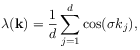 |
(15) |
into eq. (5). [5.1.2] This gives
| (16) |
where the Fourier transform of eq. (12)
was used in the last equality and the subscript
refers to the first model.
[5.1.3] Equation (16) equals the result obtained from
Fourier-Laplace transformation of the fractional Cauchy problem
defined by equations (10) and (11).
[5.1.4] Hence a CTRW-model with ![]() and the fractional
master equation describe the same random walk process in
the sense that their fundamental solutions are the same.
and the fractional
master equation describe the same random walk process in
the sense that their fundamental solutions are the same.
[5.2.1] The continuum limit ![]() was the background
and motivation for the discussion in Ref. [2].
[5.2.2] It follows from eq. (1.9) in Ref. [2] by
virtue of the continuity theorem [16] for
characteristic functions that for the first
model the continuum limit with
was the background
and motivation for the discussion in Ref. [2].
[5.2.2] It follows from eq. (1.9) in Ref. [2] by
virtue of the continuity theorem [16] for
characteristic functions that for the first
model the continuum limit with
| (17) |
leads for all fixed ![]() to
to
 |
(18) |
[5.2.3] Here the expansion ![]() has been used.
[5.2.4] Therefore the solution of the first model with
waiting time density
has been used.
[5.2.4] Therefore the solution of the first model with
waiting time density ![]() converges in the continuum limit
to the solution of the fractional diffusion equation
converges in the continuum limit
to the solution of the fractional diffusion equation
| (19) |
with initial condition analogous to eq. (11).
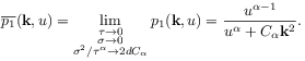
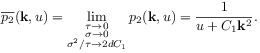
[5.3.1] Consider now the second model with waiting time density ![]() given by eq. (8).
[5.3.2] In this case
given by eq. (8).
[5.3.2] In this case
| (20) |
and
| (21) | |||
From this follows
| (22) |
showing that the continuum limit as in eq. (17) with
finite ![]() does not give rise to the propagator of fractional diffusion.
[5.3.3] On the other hand the conventional continuum limit with
does not give rise to the propagator of fractional diffusion.
[5.3.3] On the other hand the conventional continuum limit with
![]() exists and yields
exists and yields
 |
(23) |
the Gaussian propagator of ordinary diffusion with diffusion constant
![]() .
.
