2 Definition of Models
[2.3.1] Consider first the integral equation of motion for the CTRW-model
[9, 10].
[2.3.2] The probability density ![]() obeys the
integral equation
obeys the
integral equation
| (3) |
where ![]() denotes the probability
for a displacement
denotes the probability
for a displacement ![]() in each single step, and
in each single step, and ![]() is the
waiting time distribution giving the probability density
for the time interval
is the
waiting time distribution giving the probability density
for the time interval ![]() between two consecutive steps.
[2.3.3] The transition probabilities obey
between two consecutive steps.
[2.3.3] The transition probabilities obey ![]() ,
and the function
,
and the function ![]() is the survival probability at the initial
position which is related to the waiting time distribution through
is the survival probability at the initial
position which is related to the waiting time distribution through
| (4) |
[page 3, §0] Fourier-Laplace transformation leads to the solution in Fourier-Laplace space given as [10]
| (5) |
where ![]() is the Fourier-Laplace transform of
is the Fourier-Laplace transform of
![]() and similarly for
and similarly for ![]() and
and ![]() .
.
[3.1.1] Two lattice models with different waiting time density will be considered. [3.1.2] In the first model the waiting time density is chosen as the one found in [1, 2]
| (6) |
where ![]() is the characteristic time, and
is the characteristic time, and
| (7) |
is the generalized Mittag-Leffler function [14]. [3.1.3] In the second model the waiting time density is chosen as
| (8) |
where ![]() ,
, ![]() and
and ![]() is a suitable
dimensional constant.
is a suitable
dimensional constant.
[3.2.1] The waiting time density ![]() differs only little
from
differs only little
from ![]() as shown graphically in Figure 1.
as shown graphically in Figure 1.
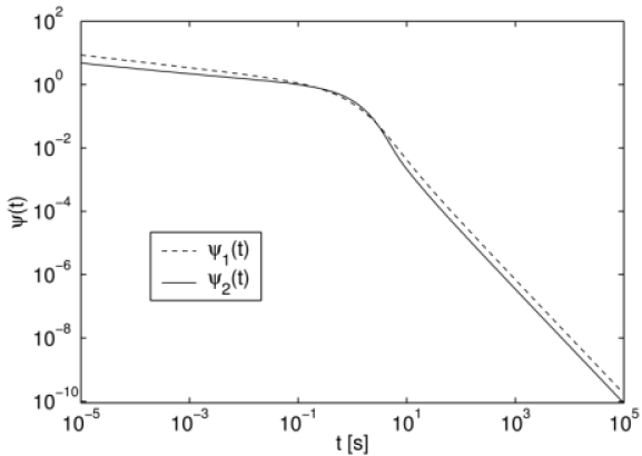
[3.2.2] Note that both models have a long time tail
of the form given in eq. (2), and
the average waiting time ![]() diverges.
diverges.
[3.3.1] For both models the spatial transition probabilities are
chosen as those for nearest-neighbour transitions (Polya walk)
on a ![]() -dimensional hypercubic lattice given as
-dimensional hypercubic lattice given as
 |
(9) |
where ![]() is the
is the ![]() -th unit basis vector generating the
lattice,
-th unit basis vector generating the
lattice, ![]() is the lattice constant and
is the lattice constant and
![]() for
for ![]() and
and
![]() for
for ![]() .
.
