3 Discussion
3.1 (Non-)locality and (in-)finite propagation speed
[335.4.1] It is the primary objective of this note to contribute
to the current debate by discussing fundamental differences
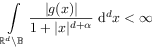
between the cases ![]() and
and ![]() in eq. (1)
for applications to experiment.
[335.4.2] The decisive difference between the cases
in eq. (1)
for applications to experiment.
[335.4.2] The decisive difference between the cases ![]() and
and ![]() is the locality of the Laplacean
is the locality of the Laplacean
![]() for
for ![]() in contrast with the nonlocality of
the fractional Laplacean
in contrast with the nonlocality of
the fractional Laplacean ![]() for
for ![]() .
.
[page 336, §1]
[336.2.1] Before discussing the (non-)locality of ![]() it seems important to distinguish it from another nonlocality
appearing in eq. (1).
[336.2.2] It is sometimes argued that also the case
it seems important to distinguish it from another nonlocality
appearing in eq. (1).
[336.2.2] It is sometimes argued that also the case ![]() shows
nonlocality in the sense that a localized initial condition
such as
shows
nonlocality in the sense that a localized initial condition
such as ![]() , vanishing everywhere
except at
, vanishing everywhere
except at ![]() for
for ![]() , spreads out instantaneously to all
, spreads out instantaneously to all ![]() such that
such that ![]() for all
for all ![]() for
for ![]() .
[336.2.3] This initially infinite “speed of propagation”
violates relativistic locality.
While this is true for all
.
[336.2.3] This initially infinite “speed of propagation”
violates relativistic locality.
While this is true for all ![]() , it concerns
the operator
, it concerns
the operator ![]() and occurs only at
and occurs only at ![]() , the initial instant.
[336.2.4] For
, the initial instant.
[336.2.4] For ![]() the operator
the operator ![]() is local
and also
is local
and also ![]() is perfectly local for all
is perfectly local for all ![]() .
[336.2.5] While an infinite propagation speed occurs also for
.
[336.2.5] While an infinite propagation speed occurs also for ![]() another violation of locality occurs in this case.
[336.2.6] This has more dramatic implications for experiment,
as will now be discussed.
another violation of locality occurs in this case.
[336.2.6] This has more dramatic implications for experiment,
as will now be discussed.
3.2 Probabilistic interpretation
[336.3.1] The fundamental difference between the cases ![]() and
and
![]() can be understood from the deep and well known relation
between the diffusion equation (1) and the
theory of stochastic processses.
[336.3.2] The probabilistic interpretation of
can be understood from the deep and well known relation
between the diffusion equation (1) and the
theory of stochastic processses.
[336.3.2] The probabilistic interpretation of ![]() is given
in terms of families of stochastic processes
is given
in terms of families of stochastic processes ![]() indexed by their starting point
indexed by their starting point ![]() through the formula
through the formula
| (5) |
where ![]() denotes the first
exit time of a path starting at
denotes the first
exit time of a path starting at ![]() and hitting the set
and hitting the set ![]() for the first
time at
for the first
time at ![]() .
[336.3.3] The brackets
.
[336.3.3] The brackets ![]() denote the expectation
value of a random variable
denote the expectation
value of a random variable ![]() evaluated for the process
evaluated for the process
![]() starting from
starting from ![]() at
at ![]() .
.
[336.4.1] For ![]() the family of stochastic processes has almost
surely continuous paths.
[336.4.2] Because of this,
a path starting from
the family of stochastic processes has almost
surely continuous paths.
[336.4.2] Because of this,
a path starting from ![]() at
at ![]() will
exit from
will
exit from ![]() when hitting
when hitting
![]() for the first time.
for the first time.
[336.5.1] For ![]() on the other hand the families of stochastic
processes have almost surely discontinuous paths that can
jump over the boundary
on the other hand the families of stochastic
processes have almost surely discontinuous paths that can
jump over the boundary ![]() .
[336.5.2] As a result the first exit occurs not at the boundary
but at some point
.
[336.5.2] As a result the first exit occurs not at the boundary
but at some point ![]() deep
in the exterior region
deep
in the exterior region ![]() .
.
[336.6.1] In applications to particle diffusion the unknown ![]() is often the concentration of atomic, molecular or tracer particles
and fractional generalizations
of Ficks law have been postulated [4, 27, 3].
[336.6.2] Note, however, that the probabilistic interpretation is
frequently not physical even for
is often the concentration of atomic, molecular or tracer particles
and fractional generalizations
of Ficks law have been postulated [4, 27, 3].
[336.6.2] Note, however, that the probabilistic interpretation is
frequently not physical even for ![]() .
[336.6.3] There are at least two possible reasons:
[336.6.4] Firstly, the underlying physical dynamics may not be stochastic.
[336.6.5] Secondly, fundamental laws of probability
[page 337, §0]
theory may be violated as for the case of heat diffusion where
.
[336.6.3] There are at least two possible reasons:
[336.6.4] Firstly, the underlying physical dynamics may not be stochastic.
[336.6.5] Secondly, fundamental laws of probability
[page 337, §0]
theory may be violated as for the case of heat diffusion where
![]() is the temperature field.
[337.0.1] In such cases the random “paths” are fictitious
as are the “particles” and their “trajectories”
in the sense that they cannot be observed directly
in an experiment.
is the temperature field.
[337.0.1] In such cases the random “paths” are fictitious
as are the “particles” and their “trajectories”
in the sense that they cannot be observed directly
in an experiment.
3.3 Stationary solutions
[337.2.1] To explore the physical consequences of the initial and boundary value problem (1),(2) and (4) it is useful to start with stationary solutions, i.e. solutions of the form
| (6) |
[337.2.2] The fractional diffusion equation then reduces to the fractional Riesz-Dirichlet problem
| (7a) | |||
| (7b) |
for suitable boundary data ![]() such that
such that
 |
(8) |
holds.
[337.3.1] The solution of the fractional Riesz-Dirichlet problem
for the case of a sphere
![]() of radius
of radius ![]() centered at
centered at ![]() is the fractional Poisson integral [16]
is the fractional Poisson integral [16]
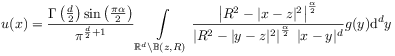 |
(9) |
for ![]() .
[337.3.2] For
.
[337.3.2] For ![]() the solution reduces to the conventional
Poisson integral
the solution reduces to the conventional
Poisson integral
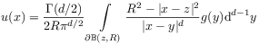 |
(10) |
for ![]() and
and
![]() for
for ![]() .
.
[337.4.1] Although the fractional Poisson formula eq. (9)
has been known for
nearly 70 years [22] its crucial difference
to (10) seems to have escaped the
attention of those scientists, who propose eq. (1)
or its variants as a mathematical model for physical phenomena.
[337.4.2] Perhaps this is due to
[page 338, §0]
the fact that many workers
assume explicitly or implicitly
“absorbing” or “killing” boundaries ![]() for all
for all ![]() .
[338.0.1] Physically this means that there are no atoms, molecules
or tracer particles
outside the spherical container
.
[338.0.1] Physically this means that there are no atoms, molecules
or tracer particles
outside the spherical container ![]() .
[338.0.2] Any particle that jumps out of
.
[338.0.2] Any particle that jumps out of ![]() is considered to be instantaneously removed
from the experiment.
[338.0.3] The environment surrounding the experimental apparatus
has to be kept absolutely clean at all times for these
boundary conditions to apply.
[338.0.4] Under these experimental conditions both equations,
eq. (9) as well as eq. (10),
agree and both predict
is considered to be instantaneously removed
from the experiment.
[338.0.3] The environment surrounding the experimental apparatus
has to be kept absolutely clean at all times for these
boundary conditions to apply.
[338.0.4] Under these experimental conditions both equations,
eq. (9) as well as eq. (10),
agree and both predict
| (11) |
for all ![]() and all
and all ![]() .
.
[338.1.1] Consider next the case when there exist regions
where the atomic, molecular
or tracer particles are not instantaneously
removed.
[338.1.2] For simplicity let there exist several small
nonoverlapping spherical containers
![]() with
with ![]() ,
,
![]() for all
for all ![]() and
and ![]() for all
for all ![]() in which particles are kept (e.g. for replenishment).
[338.1.3] This means that in these containers
in which particles are kept (e.g. for replenishment).
[338.1.3] This means that in these containers ![]() and particles jumping out of the sample region
and particles jumping out of the sample region
![]() may land in one of these containers.
[338.1.4] They are not removed until the container is filled
and a maximum concentration is reached.
[338.1.5] Let
may land in one of these containers.
[338.1.4] They are not removed until the container is filled
and a maximum concentration is reached.
[338.1.5] Let ![]() denote the maximal concentration in each
container.
[338.1.6] Assume that
denote the maximal concentration in each
container.
[338.1.6] Assume that
| (12a) | ||
| with | ||
| (12b) | ||
describes the concentration field in the region ![]() outside the sample.
[338.1.7] Other functions than
outside the sample.
[338.1.7] Other functions than ![]() with
with
![]() are possible.
[338.1.8] Assume also that
are possible.
[338.1.8] Assume also that ![]() for all
for all ![]() ,
so that in particular also
supp
,
so that in particular also
supp![]() holds.
holds.
[338.2.1] For ![]() eq. (10) shows that the solution
eq. (10) shows that the solution
![]() remains unaffected by the containers
remains unaffected by the containers ![]() and their content.
[338.2.2] For
and their content.
[338.2.2] For ![]() on the other hand the solution changes and
becomes nonzero. It is approximately
on the other hand the solution changes and
becomes nonzero. It is approximately
| (13) |
for ![]() .
[338.2.3] This result implies that for
.
[338.2.3] This result implies that for ![]() the stationary solution
inside the sample region
the stationary solution
inside the sample region ![]() depends on the location
and content of all other
containers
depends on the location
and content of all other
containers ![]() in the laboratory.
[338.2.4] The sample in
in the laboratory.
[338.2.4] The sample in ![]() [page 339, §0]
cannot be shielded or isolated from other samples in the laboratory.
[339.0.1] It should be easy to verify or falsify this prediction
in an experiment.
[page 339, §0]
cannot be shielded or isolated from other samples in the laboratory.
[339.0.1] It should be easy to verify or falsify this prediction
in an experiment.
