3 Geometric Characterizations
3.1 General Considerations
[206.2.3] A general geometric characterization of stochastic media should provide macroscopic geometric observables that allow to distinguish media with different microstructures quantitatively. [206.2.4] In general, a stochastic medium is defined as a probability distribution on a space of geometries or configurations. [206.2.5] Distributions and expectation values of geometric observables are candidates for a general geometric characterization.
[206.3.1] A general geometric characterization should fulfill four criteria to be useful in applications. [206.3.2] These four criteria were advanced in [30]. [206.3.3] First, it must be well defined. [206.3.4] This obvious requirement is sometimes violated. [206.3.5] The so called ‘‘pore size distributions’’ measured in mercury porosimetry are not geometrical observables in the sense that they cannot be determined from knowledge of the geometry alone. [206.3.6] Instead they are capillary pressure curves whose calculation involves physical quantities such as surface tension, viscosity or flooding history [30]. [206.3.7] Second, the geometric characterization should be directly accessible in experiments. [206.3.8] The experiments should be independent of the quantities to be predicted. [206.3.9] Thirdly, the numerical implementation should not require excessive amounts of data. [206.3.10] This means that the amount of data should be manageable by contemporary data processing technology. [206.3.11] Finally, a useful geometric characterization should be helpful in the exact or approximate theoretical calculations.
[206.4.1] For simplicity only two-component media will be considered throughout this paper, but most concepts can be generalized to media with an arbitrary finite number of components.
3.2 Geometric Observables
[206.4.2] Well defined geometric observables are the basis for the geometric characterization of porous media. [206.4.3] A perennial problem in all applications is to identify those [page 207, §0] macroscopic geometric observables that are relevant for distinguishing between classes of microstructures. [207.0.1] One is interested in those properties of the microstructure that influence the macroscopic physical behaviour. [207.0.2] In general this depends on the details of the physical problem, but some general properties of the microstructure such as volume fraction or porosity are known to be relevant in many situations. [207.0.3] Hadwigers theorem [23] is an example of a mathematical result that helps to identify an important class of such general geometric properties of porous media. [207.0.4] It will be seen later, however, that there exist important geometric properties that are not members of this class.
[207.1.1] A two component porous (or heterogenous) sample
![]() consists of two closed subsets
consists of two closed subsets ![]() and
and ![]() called pore space
called pore space ![]() and matrix
and matrix ![]() such that
such that ![]() .
[207.1.2] Its internal boundary is denoted as
.
[207.1.2] Its internal boundary is denoted as ![]() [207.1.3] The boundary
[207.1.3] The boundary ![]() of a set is defined as the
difference between the closure and the interior of
of a set is defined as the
difference between the closure and the interior of ![]() where the closure is the intersection of all closed
sets containing
where the closure is the intersection of all closed
sets containing ![]() and the interior is the union of
all open sets contained in
and the interior is the union of
all open sets contained in ![]() .
[207.1.4] A geometric observable
.
[207.1.4] A geometric observable ![]() is a mapping (functional) that
assigns to each admissible
is a mapping (functional) that
assigns to each admissible ![]() a real number
a real number ![]() that can be calculated from
that can be calculated from ![]() without solving a physical
boundary value problem.
[207.1.5] A functional whose evaluation requires the solution of a physical
boundary value problem will be called a physical observable.
without solving a physical
boundary value problem.
[207.1.5] A functional whose evaluation requires the solution of a physical
boundary value problem will be called a physical observable.
[207.2.1] Before discussing examples for geometric observables
it is necessary to specify the admissible geometries ![]() .
[207.2.2] The set
.
[207.2.2] The set ![]() of admissible
of admissible ![]() is defined as
the set of all finite unions of compact convex sets
[23, 61, 58, 57, 44](see also the
papers by M. Kerscher and K. Mecke in this volume).
[207.2.3] Because
is defined as
the set of all finite unions of compact convex sets
[23, 61, 58, 57, 44](see also the
papers by M. Kerscher and K. Mecke in this volume).
[207.2.3] Because ![]() is closed under unions and
intersections it is called the convex ring.
[207.2.4] The choice of
is closed under unions and
intersections it is called the convex ring.
[207.2.4] The choice of ![]() is convenient for applications
because digitized porous media can be considered as
elements from
is convenient for applications
because digitized porous media can be considered as
elements from ![]() and because continuous observables defined for
convex compact sets can be continued to all of
and because continuous observables defined for
convex compact sets can be continued to all of ![]() .
[207.2.5] The set of all compact and convex subsets of
.
[207.2.5] The set of all compact and convex subsets of ![]() is denoted as
is denoted as ![]() .
[207.2.6] For subsequent discussions the
Minkowski addition of two sets
.
[207.2.6] For subsequent discussions the
Minkowski addition of two sets ![]() is defined as
is defined as
| (8) |
[207.2.7] Multiplication of ![]() with a scalar is defined by
with a scalar is defined by
![]() for
for ![]() .
.
[207.3.1] Examples of geometric observables are the volume of ![]() or the surface area of its boundary
or the surface area of its boundary ![]() .
[207.3.2] Let
.
[207.3.2] Let
| (9) |
denote the ![]() -dimensional Lebesgue volume
of the compact convex set
-dimensional Lebesgue volume
of the compact convex set ![]() .
[207.3.3] The volume is hence a functional
.
[207.3.3] The volume is hence a functional ![]() on
on ![]() .
[207.3.4] An example of a compact convex set is the unit ball
.
[207.3.4] An example of a compact convex set is the unit ball
![]() centered at the origin
centered at the origin ![]() whose volume is
whose volume is
| (10) |
[207.3.5] Other functionals on ![]() can be constructed from the volume
by virtue of the following fact.
[207.3.6] For every compact convex
can be constructed from the volume
by virtue of the following fact.
[207.3.6] For every compact convex ![]() and every
and every
![]() there are
[page 208, §0]
numbers
there are
[page 208, §0]
numbers ![]() depending only on
depending only on ![]() such that
such that
 |
(11) |
is a polynomial in ![]() .
[208.0.1] This result is known as Steiners formula [23, 61].
[208.0.2] The numbers
.
[208.0.1] This result is known as Steiners formula [23, 61].
[208.0.2] The numbers ![]() define functionals on
define functionals on
![]() similar to the volume
similar to the volume ![]() .
[208.0.3] The quantities
.
[208.0.3] The quantities
| (12) |
are called quermassintegrals [57]. [208.0.4] From (11) one sees that
| (13) |
and from (10) that ![]() .
[208.0.5] Hence
.
[208.0.5] Hence ![]() may be viewed as half the surface area.
[208.0.6] The functional
may be viewed as half the surface area.
[208.0.6] The functional ![]() is related to the mean width
is related to the mean width ![]() defined as the mean value of the distance between a pair of
parallel support planes of
defined as the mean value of the distance between a pair of
parallel support planes of ![]() .
[208.0.7]
The relation is
.
[208.0.7]
The relation is
| (14) |
which reduces to ![]() for
for ![]() .
[208.0.8] Finally the functional
.
[208.0.8] Finally the functional ![]() is evaluated from
(11) by dividing with
is evaluated from
(11) by dividing with ![]() and taking
the limit
and taking
the limit ![]() .
[208.0.9] It follows that
.
[208.0.9] It follows that ![]() for all
for all ![]() .
[208.0.10] One extends
.
[208.0.10] One extends ![]() to all of
to all of ![]() by defining
by defining
![]() .
[208.0.11] The geometric observable
.
[208.0.11] The geometric observable ![]() is called Euler characteristic.
is called Euler characteristic.
[208.1.1] The geometric observables ![]() have several important properties.
[208.1.2] They are Euclidean invariant (i.e. invariant under rigid motions),
additive and monotone.
[208.1.3] Let
have several important properties.
[208.1.2] They are Euclidean invariant (i.e. invariant under rigid motions),
additive and monotone.
[208.1.3] Let ![]() denote the group of translations with
vector addition as group operation and let
denote the group of translations with
vector addition as group operation and let ![]() be
the matrix group of rotations in
be
the matrix group of rotations in ![]() dimensions [5].
[208.1.4] The semidirect product
dimensions [5].
[208.1.4] The semidirect product ![]() is the Euclidean
group of rigid motions in
is the Euclidean
group of rigid motions in ![]() .
[208.1.5] It is defined as the set of pairs
.
[208.1.5] It is defined as the set of pairs ![]() with
with ![]() and
and ![]() and group operation
and group operation
| (15) |
[208.1.6] An observable ![]() is called euclidean invariant
or invariant under rigid motions
if
is called euclidean invariant
or invariant under rigid motions
if
| (16) |
holds for all ![]() and all
and all ![]() .
[208.1.7] Here
.
[208.1.7] Here ![]() denotes the rotation
of
denotes the rotation
of ![]() and
and ![]() its translation.
[208.1.8] A geometric observable
its translation.
[208.1.8] A geometric observable ![]() is called additive
if
is called additive
if
| (17a) | |||
| (17b) |
holds for all ![]() with
with ![]() .
[208.1.9] Finally a functional is called monotone if for
.
[208.1.9] Finally a functional is called monotone if for ![]() with
with ![]() follows
follows ![]() .
.
[page 209, §1]
[209.1.1] The special importance of the functionals ![]() arises from
the following theorem of Hadwiger [23].
[209.1.2] A functional
arises from
the following theorem of Hadwiger [23].
[209.1.2] A functional ![]() is euclidean invariant,
additive and monotone if and only if it is a linear
combination
is euclidean invariant,
additive and monotone if and only if it is a linear
combination
| (18) |
with nonnegative constants ![]() .
[209.1.3] The condition of monotonicity can be replaced with
continuity and the theorem remains valid [23].
[209.1.4] If
.
[209.1.3] The condition of monotonicity can be replaced with
continuity and the theorem remains valid [23].
[209.1.4] If ![]() is continuous on
is continuous on ![]() , additive and euclidean invariant
it can be additively extended to the convex ring
, additive and euclidean invariant
it can be additively extended to the convex ring ![]() [58].
[209.1.5] The additive extension is unique and given by the
inclusion-exclusion formula
[58].
[209.1.5] The additive extension is unique and given by the
inclusion-exclusion formula
 |
(19) |
where ![]() denotes the family of nonempty subsets
of
denotes the family of nonempty subsets
of ![]() and
and ![]() is the number of elements
of
is the number of elements
of ![]() .
[209.1.6] In particular, the functionals
.
[209.1.6] In particular, the functionals ![]() have a unique additive extension
to the convex ring
have a unique additive extension
to the convex ring ![]() [58], which is again be denoted by
[58], which is again be denoted by ![]() .
.
[209.2.1] For a threedimensional porous sample with ![]() the extended
functionals
the extended
functionals ![]() lead to two frequently used geometric observables.
[209.2.2] The first is the porosity of a porous sample
lead to two frequently used geometric observables.
[209.2.2] The first is the porosity of a porous sample ![]() defined as
defined as
| (20) |
and the second its specific internal surface area which may be defined in view of (13) as
| (21) |
[209.2.3] The two remaining observables ![]() and
and
![]() have received less attention
in the porous media literature.
[209.2.4] The Euler characteristic
have received less attention
in the porous media literature.
[209.2.4] The Euler characteristic ![]() on
on ![]() coincides with
the identically named topological invariant.
[209.2.5] For
coincides with
the identically named topological invariant.
[209.2.5] For ![]() and
and ![]() one has
one has
![]() where
where ![]() is the number
of connectedness components of
is the number
of connectedness components of ![]() , and
, and ![]() denotes
the number of holes (i.e. bounded connectedness components
of the complement).
denotes
the number of holes (i.e. bounded connectedness components
of the complement).
3.3 Definition of Stochastic Porous Media
[209.2.6] For theoretical purposes the pore space ![]() is frequently
viewed as a random set [61, 30].
[209.2.7] In practical applications the pore space is usually discretized
because of measurement limitations and finite resolution.
[209.2.8] For the data discussed below the set
is frequently
viewed as a random set [61, 30].
[209.2.7] In practical applications the pore space is usually discretized
because of measurement limitations and finite resolution.
[209.2.8] For the data discussed below the set ![]() is a
rectangular parallelepiped whose sidelengths are
is a
rectangular parallelepiped whose sidelengths are ![]() and
and ![]() in units of the lattice constant
in units of the lattice constant ![]() (resolution)
of a simple cubic lattice.
[209.2.9] The position vectors
(resolution)
of a simple cubic lattice.
[209.2.9] The position vectors
![]() with integers
with integers ![]() are
are
[page 210, §0]
used to
label the lattice points, and ![]() is a shorthand notation for
is a shorthand notation for ![]() .
[210.0.1] Let
.
[210.0.1] Let ![]() denote a cubic volume element (voxel)
centered at the lattice site
denote a cubic volume element (voxel)
centered at the lattice site ![]() .
[210.0.2] Then the discretized sample may be represented
as
.
[210.0.2] Then the discretized sample may be represented
as ![]() .
[210.0.3] The discretized pore space
.
[210.0.3] The discretized pore space ![]() defined as
defined as
| (22) |
is an approximation to the true pore space ![]() .
[210.0.4] For simplicity it will be assumed that the
discretization does not introduce errors,
i.e. that
.
[210.0.4] For simplicity it will be assumed that the
discretization does not introduce errors,
i.e. that ![]() , and that
each voxel is either fully pore or fully matrix.
[210.0.5] This assumption may be relaxed to allow
voxel attributes such as internal surface or
other quermassintegral densities.
[210.0.6] The discretization into voxels reflects the limitations arising
from the experimental resolution of the porous structure.
[210.0.7] A discretized pore space for a bounded sample belongs
to the convex ring
, and that
each voxel is either fully pore or fully matrix.
[210.0.5] This assumption may be relaxed to allow
voxel attributes such as internal surface or
other quermassintegral densities.
[210.0.6] The discretization into voxels reflects the limitations arising
from the experimental resolution of the porous structure.
[210.0.7] A discretized pore space for a bounded sample belongs
to the convex ring ![]() if the voxels are convex and
compact.
[210.0.8] Hence, for a simple cubic discretization the pore
space belongs to the convex ring.
[210.0.9] A configuration (or microstructure)
if the voxels are convex and
compact.
[210.0.8] Hence, for a simple cubic discretization the pore
space belongs to the convex ring.
[210.0.9] A configuration (or microstructure) ![]() of a
of a
![]() -component medium may then be represented
in the simplest case by a sequence
-component medium may then be represented
in the simplest case by a sequence
| (23) |
where ![]() runs through the lattice points and
runs through the lattice points and ![]() .
[210.0.10] This representation corresponds to the simplest discretization
in which there are only two states for each voxel indicating
whether it belongs to pore space or not.
[210.0.11] In general a voxel could be characterized
by more states reflecting the microsctructure within
the region
.
[210.0.10] This representation corresponds to the simplest discretization
in which there are only two states for each voxel indicating
whether it belongs to pore space or not.
[210.0.11] In general a voxel could be characterized
by more states reflecting the microsctructure within
the region ![]() .
[210.0.12] In the simplest case there is a one-to-one correspondence
between
.
[210.0.12] In the simplest case there is a one-to-one correspondence
between ![]() and
and ![]() given by (23).
[210.0.13] Geometric observables
given by (23).
[210.0.13] Geometric observables ![]() then correspond to functions
then correspond to functions
![]() .
.
[210.1.1] As a convenient theoretical idealization it is frequently assumed that porous media are random realizations drawn from an underlying statistical ensemble. [210.1.2] A discretized stochastic porous medium is defined through the discrete probability density
| (24) |
where ![]() in the simplest case.
[210.1.3] It should be emphasized that the probability density
in the simplest case.
[210.1.3] It should be emphasized that the probability density ![]() is mainly of theoretical interest.
[210.1.4] In practice it is usually not known.
[210.1.5] An infinitely extended medium or microstructure
is called stationary or
statistically homogeneous if
is mainly of theoretical interest.
[210.1.4] In practice it is usually not known.
[210.1.5] An infinitely extended medium or microstructure
is called stationary or
statistically homogeneous if ![]() is invariant under
spatial translations.
[210.1.6] It is called isotropic if
is invariant under
spatial translations.
[210.1.6] It is called isotropic if ![]() is invariant under rotations.
is invariant under rotations.
3.4 Moment Functions and Correlation Functions
[210.1.7] A stochastic medium was defined through
its probability distribution ![]() .
[210.1.8] In practice
.
[210.1.8] In practice ![]() will be even less accessible than the
microstructure
will be even less accessible than the
microstructure ![]() itself.
[210.1.9] Partial information about
itself.
[210.1.9] Partial information about ![]() can be obtained
by measuring or calculating expectation values
of a geometric observable
can be obtained
by measuring or calculating expectation values
of a geometric observable ![]() .
[210.1.10] These are defined as
.
[210.1.10] These are defined as
| (25) |
[page 211, §0]
where the summations indicate a summation over all configurations.
[211.0.1] Consider for example the porosity ![]() defined in (20).
[211.0.2] For a stochastic medium
defined in (20).
[211.0.2] For a stochastic medium ![]() becomes a random variable.
[211.0.3] Its expectation is
becomes a random variable.
[211.0.3] Its expectation is
| (26) |
If the medium is statistically homogeneous then
| (27) |
independent of ![]() .
[211.0.4] It happens frequently that one is given only a single
sample, not an ensemble of samples.
[211.0.5] It is then necessary to invoke an ergodic hypothesis
that allows to equate spatial averages with ensemble
averages.
.
[211.0.4] It happens frequently that one is given only a single
sample, not an ensemble of samples.
[211.0.5] It is then necessary to invoke an ergodic hypothesis
that allows to equate spatial averages with ensemble
averages.
[211.1.1] The porosity is the first member in a hierarchy of
moment functions.
[211.1.2] The ![]() -th order moment function is defined generally as
-th order moment function is defined generally as
| (28) |
for ![]() .
b (This is a footnote:) b
If a voxel has other attributes besides
being pore or matrix one may define also mixed moment functions
.
b (This is a footnote:) b
If a voxel has other attributes besides
being pore or matrix one may define also mixed moment functions
![]() where
where ![]() for
for ![]() are the quermassintegral densities for the voxel at site
are the quermassintegral densities for the voxel at site ![]() .
[211.1.3] For stationary media
.
[211.1.3] For stationary media
![]() where the function
where the function ![]() depends only on
depends only on ![]() variables.
[211.1.4] Another frequently used expectation value is the correlation function
which is related to
variables.
[211.1.4] Another frequently used expectation value is the correlation function
which is related to ![]() .
[211.1.5] For a homogeneous medium it is defined as
.
[211.1.5] For a homogeneous medium it is defined as
![G({\boldsymbol{r}}_{0},{\boldsymbol{r}})=G({\boldsymbol{r}}-{\boldsymbol{r}}_{0})=\frac{\left\langle\chi\rule[-4.3pt]{0.0pt}{8.6pt}_{{\mathbb{P}}}({\boldsymbol{r}}_{0})\chi\rule[-4.3pt]{0.0pt}{8.6pt}_{{\mathbb{P}}}({\boldsymbol{r}})\right\rangle-\left\langle\phi\right\rangle^{2}}{\left\langle\phi\right\rangle(1-\left\langle\phi\right\rangle)}=\frac{S_{2}({\boldsymbol{r}}-{\boldsymbol{r}}_{0})-(S_{1}({\boldsymbol{r}}_{0}))^{2}}{S_{1}({\boldsymbol{r}}_{0})(1-S_{1}({\boldsymbol{r}}_{0}))}](mi/mi51.png) |
(29) |
where ![]() is an arbitrary reference point, and
is an arbitrary reference point, and ![]() .
[211.1.6] If the medium is isotropic then
.
[211.1.6] If the medium is isotropic then ![]() .
[211.1.7] Note that
.
[211.1.7] Note that ![]() is normalized such that
is normalized such that ![]() and
and ![]() .
.
[211.2.1] The hierarchy of moment functions ![]() , similar to
, similar to ![]() ,
is mainly of theoretical interest.
[211.2.2] For a homogeneous medium
,
is mainly of theoretical interest.
[211.2.2] For a homogeneous medium ![]() is a function of
is a function of ![]() variables.
[211.2.3] To specify
variables.
[211.2.3] To specify ![]() numerically becomes impractical
as
numerically becomes impractical
as ![]() increases.
[211.2.4] If only
increases.
[211.2.4] If only ![]() points are required along each coordinate axis
then giving
points are required along each coordinate axis
then giving ![]() would require
would require ![]() numbers.
[211.2.5] For
numbers.
[211.2.5] For ![]() this implies that already at
this implies that already at ![]() it becomes economical
to specify the microstructure
it becomes economical
to specify the microstructure ![]() directly rather than
incompletely through moment or correlation functions.
directly rather than
incompletely through moment or correlation functions.
[page 212, §1]
3.5 Contact Distributions
[212.1.1] An interesting geometric characteristic introduced and
discussed in the field of stochastic geometry are
contact distributions [18, 61, p. 206].
[212.1.2] Certain special cases of contact distributions have appeared
also in the porous media literature [20].
[212.1.3] Let ![]() be a compact test set containing the origin
be a compact test set containing the origin ![]() .
[212.1.4] Then the contact distribution is defined as the conditional
probability
.
[212.1.4] Then the contact distribution is defined as the conditional
probability
| (30) |
If one defines the random variable ![]() then
then ![]() [61].
[61].
[212.2.1] For the unit ball ![]() in three dimensions
in three dimensions ![]() is called spherical contact distribution.
[212.2.2] The quantity
is called spherical contact distribution.
[212.2.2] The quantity ![]() is then the distribution
function of the random distance from a randomly chosen
point in
is then the distribution
function of the random distance from a randomly chosen
point in ![]() to its nearest neighbour in
to its nearest neighbour in ![]() .
[212.2.3] The probability density
.
[212.2.3] The probability density
| (31) |
was discussed in [56] as a well defined alternative to the frequently used pore size distrubution from mercury porosimetry.
[212.3.1] For an oriented unit interval ![]() where
where ![]() is the a unit vector one obtains the linear
contact distribution.
[212.3.2] The linear contact distribution written as
is the a unit vector one obtains the linear
contact distribution.
[212.3.2] The linear contact distribution written as
![]() is sometimes called lineal path function [70].
[212.3.3] It is related to the chord length distribution
is sometimes called lineal path function [70].
[212.3.3] It is related to the chord length distribution ![]() defined as the probability that an interval in the intersection
of
defined as the probability that an interval in the intersection
of ![]() with a straight line containing
with a straight line containing ![]() has length smaller than
has length smaller than ![]() [30, 61, p. 208].
[30, 61, p. 208].
3.6 Local Porosity Distributions
[212.3.4] The idea of local porosity distributions is to measure
geometric observables inside compact convex subsets
![]() , and to collect the results into empirical
histograms [27].
[212.3.5] Let
, and to collect the results into empirical
histograms [27].
[212.3.5] Let ![]() denote a cube of side length
denote a cube of side length ![]() centered at the
lattice vector
centered at the
lattice vector ![]() .
[212.3.6] The set
.
[212.3.6] The set ![]() is called a measurement cell.
[212.3.7] A geometric observable
is called a measurement cell.
[212.3.7] A geometric observable ![]() , when measured inside a measurement
cell
, when measured inside a measurement
cell ![]() , is denoted as
, is denoted as ![]() and called a local
observable.
[212.3.8] An example are local Hadwiger functional densities
and called a local
observable.
[212.3.8] An example are local Hadwiger functional densities
![]() with coefficients
with coefficients ![]() as in Hadwigers theorem (18).
[212.3.9] Here the local quermassintegrals are defined using
(12) as
as in Hadwigers theorem (18).
[212.3.9] Here the local quermassintegrals are defined using
(12) as
| (32) |
for ![]() .
[212.3.10] In the following mainly the special case
.
[212.3.10] In the following mainly the special case ![]() will be of interest.
[212.3.11] For
will be of interest.
[212.3.11] For ![]() the local porosity is defined by setting
the local porosity is defined by setting ![]() ,
,
| (33) |
[page 213, §0] [213.0.1] Local densities of surface area, mean curvature and Euler characteristic may be defined analogously. [213.0.2] The local porosity distribution, defined as
| (34) |
gives the probability density to find a local porosity ![]() in the measurement cell
in the measurement cell ![]() .
[213.0.3] Here
.
[213.0.3] Here ![]() denotes the Dirac
denotes the Dirac ![]() -distribution.
[213.0.4] The support of
-distribution.
[213.0.4] The support of ![]() is the unit interval.
[213.0.5] For noncubic measurement cells
is the unit interval.
[213.0.5] For noncubic measurement cells ![]() one defines
analogously
one defines
analogously ![]() where
where
![]() is the local observable in cell
is the local observable in cell ![]() .
.
[213.1.1] The concept of local porosity distributions
c (This is a footnote:) cor more generally ‘‘local geometry distributions’’ [28, 30]
was introduced in [27] and
has been generalized in two directions [30].
[213.1.2] Firstly by admitting more than one measurement cell,
and secondly by admitting more than one geometric observable.
[213.1.3] The general ![]() -cell distribution function is defined as [30]
-cell distribution function is defined as [30]
| (35) |
for ![]() general measurement cells
general measurement cells ![]() and
and ![]() observables
observables ![]() .
[213.1.4] The
.
[213.1.4] The ![]() -cell distribution is the probability density to find
the values
-cell distribution is the probability density to find
the values ![]() of the local observable
of the local observable ![]() in cell
in cell
![]() and
and ![]() in cell
in cell ![]() and so on until
and so on until ![]() of local observable
of local observable ![]() in
in ![]() .
[213.1.5] Definition (35) is a broad generalization
of (34).
[213.1.6] This generalization is not purely academic, but was
motivated by problems of fluid flow in porous media
where not only
.
[213.1.5] Definition (35) is a broad generalization
of (34).
[213.1.6] This generalization is not purely academic, but was
motivated by problems of fluid flow in porous media
where not only ![]() but also
but also ![]() becomes
important [28].
[213.1.7] Local quermassintegrals, defined in (32),
and their linear combinations (Hadwiger functionals)
furnish important examples for local observables
in (35), and they have recently been measured
[40].
becomes
important [28].
[213.1.7] Local quermassintegrals, defined in (32),
and their linear combinations (Hadwiger functionals)
furnish important examples for local observables
in (35), and they have recently been measured
[40].
[213.2.1] The general ![]() -cell distribution is very general indeed.
[213.2.2] It even contains
-cell distribution is very general indeed.
[213.2.2] It even contains ![]() from
(24) as the special case
from
(24) as the special case ![]() and
and ![]() with
with
![]() .
[213.2.3] More precisely one has
.
[213.2.3] More precisely one has
| (36) |
because in that case ![]() if
if ![]() and
and
![]() for
for ![]() .
[213.2.4] In this way it is seen that the very definition of a stochastic
geometry is related to local porosity distributions
(or more generally local geometry distributions).
[213.2.5] As a consequence the general
.
[213.2.4] In this way it is seen that the very definition of a stochastic
geometry is related to local porosity distributions
(or more generally local geometry distributions).
[213.2.5] As a consequence the general ![]() -cell distribution
-cell distribution
![]() is again mainly of theoretical
interest, and usually unavailable for practical computations.
is again mainly of theoretical
interest, and usually unavailable for practical computations.
[213.3.1] Expectation values with respect to ![]() have generalizations to averages with respect to
have generalizations to averages with respect to ![]() .
[213.3.2] Averaging with respect to
.
[213.3.2] Averaging with respect to ![]() will be denoted by an overline.
[213.3.3] In the
will be denoted by an overline.
[213.3.3] In the
[page 214, §0]
special case ![]() and
and ![]() with
with ![]() one finds [30]
one finds [30]
| (37) |
thereby identifying the moment functions of order ![]() as averages with respect to an
as averages with respect to an ![]() -cell distribution.
-cell distribution.
[214.1.1] For practical applications the ![]() -cell local porosity
distributions
-cell local porosity
distributions ![]() and their analogues for other
quermassintegrals are of greatest interest.
[214.1.2] For a homogeneous medium the local porosity distribution obeys
and their analogues for other
quermassintegrals are of greatest interest.
[214.1.2] For a homogeneous medium the local porosity distribution obeys
| (38) |
for all lattice vectors ![]() , i.e. it is independent of
the placement of the measurement cell.
[214.1.3] A disordered medium with substitutional disorder [71]
may be viewed as a stochastic geometry obtained by placing
random elements at the cells or sites of a fixed regular
substitution lattice.
[214.1.4] For a substitutionally disordered medium
the local porosity distribution
, i.e. it is independent of
the placement of the measurement cell.
[214.1.3] A disordered medium with substitutional disorder [71]
may be viewed as a stochastic geometry obtained by placing
random elements at the cells or sites of a fixed regular
substitution lattice.
[214.1.4] For a substitutionally disordered medium
the local porosity distribution ![]() is a periodic function of
is a periodic function of ![]() whose
period is the lattice constant of the substitution
lattice.
[214.1.5] For stereological issues in the measurement of
whose
period is the lattice constant of the substitution
lattice.
[214.1.5] For stereological issues in the measurement of ![]() from thin sections see [64].
from thin sections see [64].
[214.2.1] Averages with respect to ![]() are denoted by an overline.
[214.2.2] For a homogeneous medium the average local porosity is found as
are denoted by an overline.
[214.2.2] For a homogeneous medium the average local porosity is found as
| (39) |
[page 215, §0]
independent of ![]() and
and ![]() .
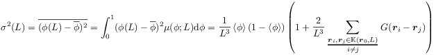
[215.0.1] The variance of local porosities for a homogeneous medium
defined in the first equality
.
[215.0.1] The variance of local porosities for a homogeneous medium
defined in the first equality
 |
(40) |
is related to the correlation function as given in the second equality [30]. [215.0.2] The skewness of the local porosity distribution is defined as the average
| (41) |
[215.1.1] The limits ![]() and
and ![]() of small resp. large
measurement cells are of special interest.
[215.1.2] In the first case one reaches the limiting resolution
at
of small resp. large
measurement cells are of special interest.
[215.1.2] In the first case one reaches the limiting resolution
at ![]() and finds for a homogeneous medium [27, 30]
and finds for a homogeneous medium [27, 30]
| (42) |
[215.1.3] The limit ![]() is more intricate because it requires
also the limit
is more intricate because it requires
also the limit ![]() .
[215.1.4] For a homogeneous medium (40)
shows
.
[215.1.4] For a homogeneous medium (40)
shows ![]() for
for ![]() and this suggests
and this suggests
| (43) |
[215.1.5] For macroscopically heterogeneous media, however,
the limiting distribution may deviate from this result
[30].
[215.1.6] If (43) holds then in both limits the geometrical
information contained in ![]() reduces to the single number
reduces to the single number
![]() .
[215.1.7] If (42) and (43) hold there exists a special
length scale
.
[215.1.7] If (42) and (43) hold there exists a special
length scale ![]() defined as
defined as
| (44) |
at which the ![]() -components at
-components at ![]() and
and ![]() vanish.
[215.1.8] In the examples below the length
vanish.
[215.1.8] In the examples below the length ![]() is a measure for
the size of pores.
is a measure for
the size of pores.
[215.2.1] The ensemble picture underlying the definition of a stochastic medium is an idealization. [215.2.2] In practice one is given only a single realization and has to resort to an ergodic hypothesis for obtaining an estimate of the local porosity distributions. [215.2.3] In the examples below the local porosity distribution is estimated by
| (45) |
where ![]() is the number of placements of the measurement
cell
is the number of placements of the measurement
cell ![]() .
[215.2.4] Ideally the measurement cells should be far apart or at
least nonoverlapping, but in
.
[215.2.4] Ideally the measurement cells should be far apart or at
least nonoverlapping, but in
[page 216, §0]
practice this restriction
cannot be observed because the samples are not large enough.
[216.0.1] In the results presented below ![]() is placed on
all lattice sites which are at least a distance
is placed on
all lattice sites which are at least a distance ![]() from
the boundary of
from
the boundary of ![]() .
[216.0.2] This allows for
.
[216.0.2] This allows for
| (46) |
placements of ![]() in a sample with side lengths
in a sample with side lengths ![]() .
[216.0.3] The use of
.
[216.0.3] The use of ![]() instead of
instead of ![]() can lead to deviations due to
violations of the ergodic hypothesis or simply due to oversampling
the central regions of
can lead to deviations due to
violations of the ergodic hypothesis or simply due to oversampling
the central regions of ![]() [10, 11].
[10, 11].
3.7 Local Percolation Probabilities
[216.0.4] Transport and propagation in porous media are controlled by the connectivity of the pore space. [216.0.5] Local percolation probabilities characterize the connectivity [27]. [216.0.6] Their calculation requires a threedimensional pore space representation, and early results were restricted to samples reconstructed laboriously from sequential thin sectioning [32].
[216.1.1] Consider the functional ![]() defined by
defined by
| (47) |
where ![]() are two compact
convex sets with
are two compact
convex sets with ![]() and
and
![]() ,
and ‘‘
,
and ‘‘![]() in
in ![]() ’’ means that
there is a path connecting
’’ means that
there is a path connecting ![]() and
and ![]() that lies
completely in
that lies
completely in ![]() .
[216.1.2] In the examples below the sets
.
[216.1.2] In the examples below the sets ![]() and
and ![]() correspond to
opposite faces of the sample, but in general other choices
are allowed.
[216.1.3] Analogous to
correspond to
opposite faces of the sample, but in general other choices
are allowed.
[216.1.3] Analogous to ![]() defined for the whole sample one defines
for a measurement cell
defined for the whole sample one defines
for a measurement cell
| (48) |
where ![]() and
and ![]() denote those two faces of
denote those two faces of
![]() that are normal to the
that are normal to the ![]() direction.
[216.1.4] Similarly
direction.
[216.1.4] Similarly ![]() denote the faces of
denote the faces of ![]() normal to the
normal to the ![]() - and
- and ![]() -directions.
[216.1.5] Two additional percolation observables
-directions.
[216.1.5] Two additional percolation observables ![]() and
and ![]() are introduced by
are introduced by
| (49) | |||
| (50) |
[216.1.6] ![]() indicates that the cell is percolating in
all three directions while
indicates that the cell is percolating in
all three directions while ![]() indicates
percolation in
indicates
percolation in ![]() - or
- or ![]() -
- ![]() -direction.
[216.1.7] The local percolation probabilities are defined as
-direction.
[216.1.7] The local percolation probabilities are defined as
| (51) |
[page 217, §0] where
| (52) |
[217.0.1] The local percolation probability ![]() gives
the fraction of measurement cells of sidelength
gives
the fraction of measurement cells of sidelength ![]() with
local porosity
with
local porosity ![]() that are percolating in the ‘‘
that are percolating in the ‘‘![]() ’’-direction.
[217.0.2] The total fraction of cells percolating along the ‘‘
’’-direction.
[217.0.2] The total fraction of cells percolating along the ‘‘![]() ’’-direction
is then obtained by integration
’’-direction
is then obtained by integration
| (53) |
[217.0.3] This geometric observable is a quantitative measure for the number
of elements that have to be percolating if the pore
space geometry is approximated by a substitutionally
disordered lattice or network model.
[217.0.4] Note that neither ![]() nor
nor ![]() are additive
functionals, and hence local percolation probabilities
have nothing to do with Hadwigers theorem.
are additive
functionals, and hence local percolation probabilities
have nothing to do with Hadwigers theorem.
[217.1.1] It is interesting that there is a relation between
the local percolation probabilities and the local Euler
characteristic ![]() .
[217.1.2] The relation arises from the observation that the voxels
.
[217.1.2] The relation arises from the observation that the voxels
![]() are closed, convex sets, and hence for any two voxels
are closed, convex sets, and hence for any two voxels
![]() the Euler characteristic of their intersection
the Euler characteristic of their intersection
| (54) |
indicates whether two voxels are nearest neighbours.
[217.1.3] A measurement cell ![]() contains
contains ![]() voxels.
[217.1.4] It is then possible to construct a
voxels.
[217.1.4] It is then possible to construct a ![]() -matrix
-matrix
![]() with matrix elements
with matrix elements
| (55) | |||
| (56) |
where ![]() and the
sets
and the
sets ![]() and
and ![]() are two opposite
faces of the measurement cell.
[217.1.5] The rows in the matrix
are two opposite
faces of the measurement cell.
[217.1.5] The rows in the matrix ![]() correspond to voxels while
the columns correspond to voxel pairs.
[217.1.6] Define the matrix
correspond to voxels while
the columns correspond to voxel pairs.
[217.1.6] Define the matrix ![]() where
where ![]() is the transpose of
is the transpose of ![]() .
[217.1.7] The diagonal elements
.
[217.1.7] The diagonal elements ![]() give the number of
voxels to which the voxel
give the number of
voxels to which the voxel ![]() is connected.
[217.1.8] A matrix element
is connected.
[217.1.8] A matrix element ![]() differs from zero
if and only if
differs from zero
if and only if ![]() and
and ![]() are connected.
[217.1.9] Hence the matrix
are connected.
[217.1.9] Hence the matrix ![]() reflects the local
connectedness of the pore space around a single voxel.
[217.1.10] Sufficiently high powers of
reflects the local
connectedness of the pore space around a single voxel.
[217.1.10] Sufficiently high powers of ![]() provide information about the global
connectedness of
provide information about the global
connectedness of ![]() .
[217.1.11] One finds
.
[217.1.11] One finds
| (57) |
where ![]() is the matrix element in the upper right
hand corner and
is the matrix element in the upper right
hand corner and ![]() is arbitrary subject to the condition
is arbitrary subject to the condition ![]() .
[217.1.12] The set
.
[217.1.12] The set ![]() can always be decomposed uniquely
into pairwise disjoint connectedness components (clusters)
can always be decomposed uniquely
into pairwise disjoint connectedness components (clusters)
[page 218, §0]
![]() whose number is given by the rank of
whose number is given by the rank of ![]() .
[218.0.1] Hence
.
[218.0.1] Hence
| (58) |
provides an indirect connection between the local
Euler characteristic and the local percolation probabilities
mediated by the matrix ![]() .
d (This is a footnote:) dFor percolation systems it has been conjectured that
the zero of the Euler characteristic as a function of
the occupation probability is an approximation
to the percolation threshold [45])
.
d (This is a footnote:) dFor percolation systems it has been conjectured that
the zero of the Euler characteristic as a function of
the occupation probability is an approximation
to the percolation threshold [45])
