5 Quantitative Comparison of Microstructures
[page 228, §1]
5.1 Conventional Observables and Correlation Functions
[228.1.1] Table 2 gives an overview of several
geometric properties for the four microstructures
discussed in the previous section.
[228.1.2] Samples GF and SA were constructed to have the same
correlation function as sample EX.
[228.1.3] Figure 7 shows the directionally averaged
correlation functions
![]() of all four microstructures
where the notation
of all four microstructures
where the notation ![]() was used.
was used.
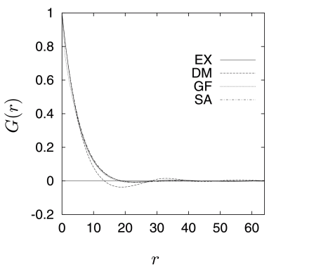
[228.2.1] The Gaussian field reconstruction ![]() is
not perfect and differs from
is
not perfect and differs from ![]() for small
for small ![]() .
[228.2.2] The discrepancy at small
.
[228.2.2] The discrepancy at small ![]() reflects the quality of the linear
filter, and it is also responsible for the differences of the
porosity and specific internal surface.
[228.2.3] Also, by construction,
reflects the quality of the linear
filter, and it is also responsible for the differences of the
porosity and specific internal surface.
[228.2.3] Also, by construction, ![]() is not expected to
equal
is not expected to
equal ![]() for
for ![]() larger than 30.
[228.2.4] Although the reconstruction method of sample
larger than 30.
[228.2.4] Although the reconstruction method of sample ![]() is
intrinsically anisotropic the correlation function of
sample SA agrees also in the diagonal directions with that
of sample EX.
[228.2.5] Sample
is
intrinsically anisotropic the correlation function of
sample SA agrees also in the diagonal directions with that
of sample EX.
[228.2.5] Sample ![]() while matching the porosity and
grain size distribution was not constructed to match
also the correlation function.
[228.2.6] As a consequence
while matching the porosity and
grain size distribution was not constructed to match
also the correlation function.
[228.2.6] As a consequence ![]() differs clearly from the rest.
[228.2.7] It reflects the grain structure of the model by becoming
negative.
[228.2.8]
differs clearly from the rest.
[228.2.7] It reflects the grain structure of the model by becoming
negative.
[228.2.8] ![]() is also anisotropic.
is also anisotropic.
[page 229, §1] [229.1.1] If two samples have the same correlation function they are expected to have also the same specific internal surface as calculated from
| (67) |
[229.1.2] The specific internal surface area calculated from this formula is given in Table 2 for all four microstructures.
[229.2.1] If one defines a decay length by the first zero
of the correlation function then the decay length
is roughly ![]() for samples EX, GF and SA.
[229.2.2] For sample DM it is somewhat smaller mainly in the
for samples EX, GF and SA.
[229.2.2] For sample DM it is somewhat smaller mainly in the ![]() -
and
-
and ![]() -direction.
[229.2.3] The correlation length, which will be of the order of the decay
length, is thus relatively large compared
to the system size.
[229.2.4] Combined with the fact that the percolation threshold for continuum
systems is typically around
-direction.
[229.2.3] The correlation length, which will be of the order of the decay
length, is thus relatively large compared
to the system size.
[229.2.4] Combined with the fact that the percolation threshold for continuum
systems is typically around ![]() this might explain why models
GF and SA are connected in spite of their low value of the porosity.
this might explain why models
GF and SA are connected in spite of their low value of the porosity.
[229.3.1] In summary, the samples ![]() and
and ![]() were
constructed to be indistinguishable with respect to
porosity and correlations from
were
constructed to be indistinguishable with respect to
porosity and correlations from ![]() .
[229.3.2] Sample SA comes close to this goal.
[229.3.3] The imperfection of the reconstruction method for
sample GF accounts for the deviations of its
correlation function at small
.
[229.3.2] Sample SA comes close to this goal.
[229.3.3] The imperfection of the reconstruction method for
sample GF accounts for the deviations of its
correlation function at small ![]() from that of sample EX.
[229.3.4] Although the difference in
porosity and specific surface is much bigger between
samples SA and GF than between samples SA and
EX sample SA is in fact more similar to GF than
to EX in a way that can be quantified using local
porosity analysis.
[229.3.5] Traditional characteristics such as porosity,
specific surface and correlation functions are insufficient
to distinguish different microstructures.
[229.3.6] Visual inspection of the pore space
indicates that samples GF and SA have a similar
structure which, however, differs from the structure
of sample EX.
[229.3.7] Although sample DM resembles sample EX more closely
with respect to surface roughness it differs visibly
in the shape of the grains.
from that of sample EX.
[229.3.4] Although the difference in
porosity and specific surface is much bigger between
samples SA and GF than between samples SA and
EX sample SA is in fact more similar to GF than
to EX in a way that can be quantified using local
porosity analysis.
[229.3.5] Traditional characteristics such as porosity,
specific surface and correlation functions are insufficient
to distinguish different microstructures.
[229.3.6] Visual inspection of the pore space
indicates that samples GF and SA have a similar
structure which, however, differs from the structure
of sample EX.
[229.3.7] Although sample DM resembles sample EX more closely
with respect to surface roughness it differs visibly
in the shape of the grains.
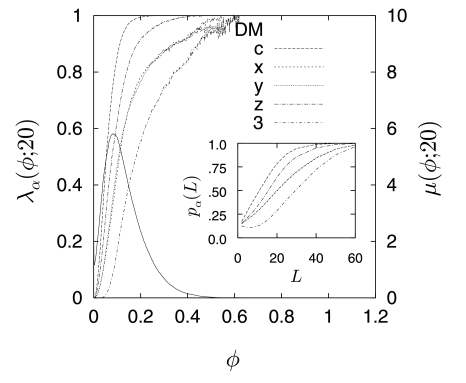
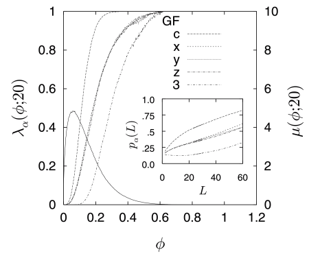
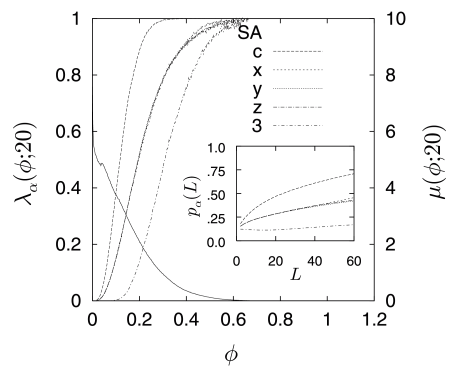
5.2 Local Porosity Analysis
[229.3.8] The differences in visual appearance of the four
microstructures can be quantified using the geometric
observables ![]() and
and ![]() from local porosity theory.
[229.3.9] The local porosity distributions
from local porosity theory.
[229.3.9] The local porosity distributions ![]() of the four samples
at
of the four samples
at ![]() are displayed as the solid lines in Figures
8a through 8d.
[229.3.10] The ordinates for these curves are plotted on the right vertical
axis.
are displayed as the solid lines in Figures
8a through 8d.
[229.3.10] The ordinates for these curves are plotted on the right vertical
axis.
[229.4.1] The figures show that the original sample exhibits stronger
porosity fluctuations than the three model samples except for
sample SA which comes close.
[229.4.2] Sample DM has the narrowest distribution which
indicates that it is most homogeneous.
[229.4.3] Figures 8a–8d show also that the ![]() -function
component at the origin,
-function
component at the origin, ![]() , is largest for sample EX, and
smallest for sample GF.
[229.4.4] For samples DM and SA the values of
, is largest for sample EX, and
smallest for sample GF.
[229.4.4] For samples DM and SA the values of ![]() are intermediate
and comparable.
[229.4.5] Plotting
are intermediate
and comparable.
[229.4.5] Plotting ![]() as a function of
as a function of ![]() shows that
this remains true for all
shows that
this remains true for all ![]() .
[229.4.6] These results indicate that the experimental sample EX is
more strongly heterogeneous than the models, and that large
regions of matrix space occur more frequently in sample EX.
[229.4.7] A similar conclusion may be drawn from the variance of
local porosity
.
[229.4.6] These results indicate that the experimental sample EX is
more strongly heterogeneous than the models, and that large
regions of matrix space occur more frequently in sample EX.
[229.4.7] A similar conclusion may be drawn from the variance of
local porosity
[page 230, §0]
[page 231, §0]
[page 232, §0]
fluctuations which will be studied below.
[232.0.1] The conclusion is also consistent with the results for ![]() shown in Table 2.
[232.0.2]
shown in Table 2.
[232.0.2] ![]() gives the sidelength of the largest cube that can be
fit into matrix space, and thus
gives the sidelength of the largest cube that can be
fit into matrix space, and thus
![]() may be viewed as a measure for the size of the largest grain.
[232.0.3] Table 2 shows that the experimental sample has a larger
may be viewed as a measure for the size of the largest grain.
[232.0.3] Table 2 shows that the experimental sample has a larger
![]() than all the models.
[232.0.4] It is interesting to note that plotting
than all the models.
[232.0.4] It is interesting to note that plotting ![]() versus
versus
![]() also shows that the curve for the experimental sample
lies above those for the other samples for all
also shows that the curve for the experimental sample
lies above those for the other samples for all ![]() .
[232.0.5] Thus, also the size of the largest pore and the pore space
heterogeneity are largest for sample EX.
[232.0.6] If
.
[232.0.5] Thus, also the size of the largest pore and the pore space
heterogeneity are largest for sample EX.
[232.0.6] If ![]() is plotted for all four samples one
finds two groups.
[232.0.7] The first group is formed by samples EX and DM,
the second by samples GF and SA.
[232.0.8] Within each group the curves
is plotted for all four samples one
finds two groups.
[232.0.7] The first group is formed by samples EX and DM,
the second by samples GF and SA.
[232.0.8] Within each group the curves ![]() nearly overlap,
but they differ strongly between them.
nearly overlap,
but they differ strongly between them.
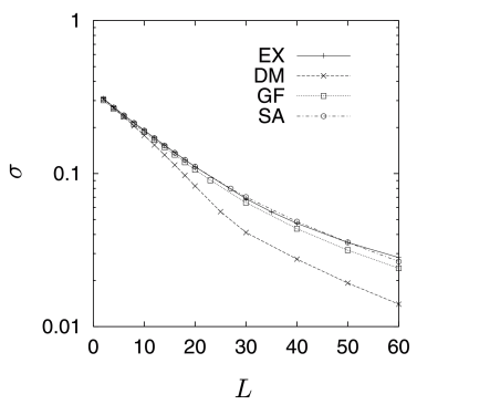
[232.1.2] Figure 9 shows the variance of the local
porosity fluctuations, defined in (40) as function
of ![]() .
[232.1.3] The variances for all samples indicate an approach to a
.
[232.1.3] The variances for all samples indicate an approach to a
![]() -distribution according to (43).
[232.1.4] Again sample DM is most homogeneous in the sense that
its variance is smallest.
[232.1.5] The agreement between samples EX, GF and SA reflects the
agreement of their correlation functions, and is expected
by virtue of eq. (40).
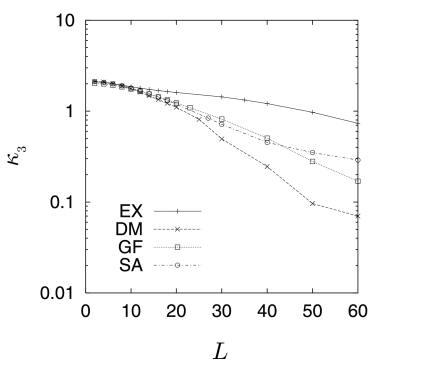
[232.1.6] Figure 10 shows the skewness as a function of
-distribution according to (43).
[232.1.4] Again sample DM is most homogeneous in the sense that
its variance is smallest.
[232.1.5] The agreement between samples EX, GF and SA reflects the
agreement of their correlation functions, and is expected
by virtue of eq. (40).
[232.1.6] Figure 10 shows the skewness as a function of ![]() calculated from
(41).
[232.1.7]
calculated from
(41).
[232.1.7] ![]() characterizes the asymmetry of the distribution,
and the difference between the most probable local
porosity and its average.
[232.1.8] Again samples GF and SA behave similarly, but sample DM and
sample EX differ from each other, and from the rest.
characterizes the asymmetry of the distribution,
and the difference between the most probable local
porosity and its average.
[232.1.8] Again samples GF and SA behave similarly, but sample DM and
sample EX differ from each other, and from the rest.
[page 233, §1]
[233.1.1] At ![]() the local porosity distributions
the local porosity distributions ![]() show small spikes at equidistantly spaced porosities for
samples EX and DM, but not for samples GF and SA.
[233.1.2] The spikes indicate that models EX and DM have a smoother
surface than models GF and SA.
[233.1.3] For smooth surfaces
and small measurement cell size porosities
corresponding to an interface intersecting the measurement
cell produce a finite probability for certain porosities
because the discretized interface allows only certain
volume fractions.
[233.1.4] In general whenever a certain porosity occurrs with
finite probability this leads to spikes in
show small spikes at equidistantly spaced porosities for
samples EX and DM, but not for samples GF and SA.
[233.1.2] The spikes indicate that models EX and DM have a smoother
surface than models GF and SA.
[233.1.3] For smooth surfaces
and small measurement cell size porosities
corresponding to an interface intersecting the measurement
cell produce a finite probability for certain porosities
because the discretized interface allows only certain
volume fractions.
[233.1.4] In general whenever a certain porosity occurrs with
finite probability this leads to spikes in ![]() .
.
5.3 Local Percolation Analysis
[233.1.5] Visual inspection of Figures 1 through 4 does not reveal the degree of connectivity of the various samples. [233.1.6] A quantitative characterization of connectivity is provided by local percolation probabilities [27, 10], and it is here that the samples differ most dramatically.
[233.2.1] The samples EX, DM , GF and SA are globally connected in all
three directions.
[233.2.2] This, however, does not imply that they have similar
connectivity.
[233.2.3] The last line in Table 2 gives the fraction of blocking
cells at the porosity ![]() and for
and for ![]() .
[233.2.4] It gives a first indication that the connectivity of samples DM and GF
is, in fact, much poorer than that of the experimental sample EX.
.
[233.2.4] It gives a first indication that the connectivity of samples DM and GF
is, in fact, much poorer than that of the experimental sample EX.
[233.3.1] Figures 8a through 8d give a more complete
account of the situation by exhibiting ![]() for
for ![]() for all four samples.
[233.3.2] First one notes that sample DM is strongly anisotropic in its
connectivity.
[233.3.3] It has a higher connectivity
for all four samples.
[233.3.2] First one notes that sample DM is strongly anisotropic in its
connectivity.
[233.3.3] It has a higher connectivity
[page 234, §0]
in the ![]() -direction than
in the
-direction than
in the ![]() - or
- or ![]() -direction.
[234.0.1] This was found to be partly due to the coarse grid used in the
sedimentation algorithm [47].
[234.0.2]
-direction.
[234.0.1] This was found to be partly due to the coarse grid used in the
sedimentation algorithm [47].
[234.0.2] ![]() for sample DM differs from that of sample EX
although their correlation functions in the
for sample DM differs from that of sample EX
although their correlation functions in the ![]() -direction are
very similar.
[234.0.3] The
-direction are
very similar.
[234.0.3] The ![]() -functions for samples EX and DM rise much
more rapidly than those for samples GF and SA.
[234.0.4] The inflection point of the
-functions for samples EX and DM rise much
more rapidly than those for samples GF and SA.
[234.0.4] The inflection point of the ![]() -curves for samples
EX and DM is much closer to the most probable porosity
(peak) than in samples GF and SA.
[234.0.5] All of this indicates that connectivity in
cells with low porosity is higher for samples EX and DM than
for samples GF and SA.
[234.0.6] In samples GF and SA only cells with high porosity are
percolating on average.
[234.0.7] In sample DM the curves
-curves for samples
EX and DM is much closer to the most probable porosity
(peak) than in samples GF and SA.
[234.0.5] All of this indicates that connectivity in
cells with low porosity is higher for samples EX and DM than
for samples GF and SA.
[234.0.6] In samples GF and SA only cells with high porosity are
percolating on average.
[234.0.7] In sample DM the curves ![]() and
and ![]() show strong fluctuations for
show strong fluctuations for ![]() at values
of
at values
of ![]() much larger than the
much larger than the ![]() or
or ![]() .
[234.0.8] This indicates a large number of high porosity cells which are
nevertheless blocked.
[234.0.9] The reason for this is perhaps that the linear compaction process
in the underlying model blocks
horizontal pore throats and decreases horizontal spatial continuity
more effectively than in the vertical direction, as shown in
[4], Table 1 p. 142.
.
[234.0.8] This indicates a large number of high porosity cells which are
nevertheless blocked.
[234.0.9] The reason for this is perhaps that the linear compaction process
in the underlying model blocks
horizontal pore throats and decreases horizontal spatial continuity
more effectively than in the vertical direction, as shown in
[4], Table 1 p. 142.
[234.1.1] The absence of spikes in ![]() for samples GF and SA combined
with the fact that cells with average porosity (
for samples GF and SA combined
with the fact that cells with average porosity (![]() )
are rarely percolating suggests that these samples have a random
morphology similar to percolation.
)
are rarely percolating suggests that these samples have a random
morphology similar to percolation.
[234.2.1] The insets in Figures 8a through 8d show the
functions ![]() for
for
![]() for each sample calculated from (53).
[234.2.2] The curves for samples EX and DM are similar but differ
from those for samples GF and SA.
[234.2.3] Figure 11 exhibits the curves
for each sample calculated from (53).
[234.2.2] The curves for samples EX and DM are similar but differ
from those for samples GF and SA.
[234.2.3] Figure 11 exhibits the curves ![]() of all
four samples in a single figure.
[234.2.4] The samples fall into two groups {EX,DM} and {GF,SA}
that behave very differently.
[234.2.5] Figure 11
of all
four samples in a single figure.
[234.2.4] The samples fall into two groups {EX,DM} and {GF,SA}
that behave very differently.
[234.2.5] Figure 11
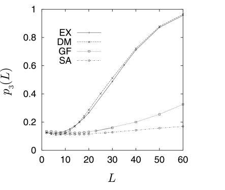
[page 235, §0] suggests that reconstruction methods [1, 70] based on correlation functions do not reproduce the connectivity properties of porous media. [235.0.1] As a consequence, one expects that also the physical transport properties will differ from the experimental sample, and it appears questionable whether a pure correlation function reconstruction can produce reliable models for the prediction of transport.
[235.1.1] Preliminary results [42] indicate that these conclusions remain unaltered if the linear and/or spherical contact distribution are incorporated into the simulated annealing reconstruction. [235.1.2] It was suggested in [70] that the linear contact distribution should improve the connectivity properties of the reconstruction, but the reconstructions performed by [42] seem not to confirm this expectation.
