VI Model Calculations
[68.1.2.1] This section returns to eq. (3.2)
and presents numerical solutions.
[68.1.2.2] This is intended as a case study exploring the relationship
between the statistics of local geometries
and bulk dielectric behavior.
[68.1.2.3] The main focus will be on dielectric enhancement.
[68.1.2.4] To solve eq. (3.2) for ![]() ,
one must know the geometric input functions
,
one must know the geometric input functions ![]() ,
, ![]() and local dielectric responses
and local dielectric responses ![]() ,
, ![]() .
[68.1.2.5] Unfortunately, no experimental data are available at present,[27]
and geometric modeling has to be used instead.
.
[68.1.2.5] Unfortunately, no experimental data are available at present,[27]
and geometric modeling has to be used instead.
A Local dielectric response
[68.1.3.1] The hypothesis of local simplicity states that the local geometries are simple and that the effective local dielectric constants are insensitive to geometrical details other than local porosity. [68.1.3.2] The simplest isotropic local geometry is spherical. [68.2.0.1] For conducting local geometries, a water-coated spherical rock grain will serve as the local model. [68.2.0.2] For blocking geometries a rock-coated spherical water pore is employed. [68.2.0.3] In the notation of Sec. IV, this means
| (6.1) | |||
| (6.2) |
[68.2.0.4] In the low-frequency limit, one obtains for the conducting geometry
| (6.3) |
thereby identifying ![]() in eq. (4.8) as
in eq. (4.8) as ![]() .
[68.2.0.5] The real dielectric constant is found as
.
[68.2.0.5] The real dielectric constant is found as
| (6.4) |
[68.2.0.6] For the blocking geometry, the dc limit gives ![]() ,
in agreement with eq. (4.6), and
,
in agreement with eq. (4.6), and
| (6.5) |
for ![]() , identifying
, identifying ![]() in eq. (4.9),
and
in eq. (4.9),
and ![]() , for
, for ![]() .
[68.2.0.7] Note the presence of the thin-plate divergence in the
.
[68.2.0.7] Note the presence of the thin-plate divergence in the ![]() limit.
limit.
B Local porosity distribution
[68.2.1.1] It was mentioned repeatedly that no experimental data for ![]() are available to the author at present.
[68.2.1.2] A qualitative guideline for porous media resulting
from spinodal decomposition might be the shape
of the order-parameter distribution calculated in Ref. [28]
which suggests in particular that
are available to the author at present.
[68.2.1.2] A qualitative guideline for porous media resulting
from spinodal decomposition might be the shape
of the order-parameter distribution calculated in Ref. [28]
which suggests in particular that ![]() can be bimodal.
can be bimodal.
[68.2.2.1] For the subsequent calculations,
a simple mixture of two ![]() distributions has been used.
[68.2.2.2] The analytic expression reads
distributions has been used.
[68.2.2.2] The analytic expression reads
| (6.6) |
where ![]() ,
, ![]() ,
, ![]() and
and ![]() denotes Euler’s
denotes Euler’s ![]() function.
[68.2.2.3] The bulk porosity is then given as
function.
[68.2.2.3] The bulk porosity is then given as
| (6.7) |
[68.2.2.4] For ![]() , the
, the ![]() densities are bell shaped,
and for
densities are bell shaped,
and for ![]() they diverge at the limits.
they diverge at the limits.
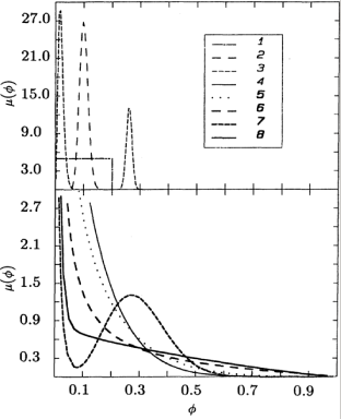
[68.2.3.1] Eight different local porosity distributions
are compared in the calculations.
[68.2.3.2] All of them are chosen such that they give
the same bulk porosity ![]() .
[68.2.3.3] The values of the parameters are listed in Table 1,
and the densities
[page 69, §0]
themselves are displayed graphically in fig. 1.
[69.1.0.1] Each distribution is identified by a number
and a line style as indicated in the inset of Fig. 1.
.
[68.2.3.3] The values of the parameters are listed in Table 1,
and the densities
[page 69, §0]
themselves are displayed graphically in fig. 1.
[69.1.0.1] Each distribution is identified by a number
and a line style as indicated in the inset of Fig. 1.
![]() (
(![]() ) are the partial porosities
) are the partial porosities
![]() in eq. (6.7).
[69.1.0.2] The uniform distribution carries number
in eq. (6.7).
[69.1.0.2] The uniform distribution carries number ![]() and is identified by a thin dot-dashed line.
[69.1.0.3] Number
and is identified by a thin dot-dashed line.
[69.1.0.3] Number ![]() represents the strongly peaked case
and is identified by a wide dashed line,
and so on.
represents the strongly peaked case
and is identified by a wide dashed line,
and so on.
| Curve No. | 1 | 2 | 3 | 4 | 5 | 6 | 7 | 8 |
|---|---|---|---|---|---|---|---|---|
| 1 | 1 | 2/3 | 1 | 1 | 1 | 2/3 | 2/3 | |
| 1.0 | 360.0 | 191.1 | 7.2 | 4.5 | 1.8 | 28.8 | 58.6 | |
| 1.000 | 40.000 | 3.900 | 0.800 | 0.500 | 0.200 | 0.087 | 0.176 | |
| 1423.0 | 13.9 | 2.24 | ||||||
| 500.00 | 6.00 | 0.96 | ||||||
| 0.1 | 0.1 | 0.02 | 0.1 | 0.1 | 0.1 | 0.003 | 0.003 | |
| 0.26 | 0.294 | 0.294 | ||||||
| 0.00333 | 0.00024 | 0.00010 | 0.00010 | 0.01500 | 0.03000 | 0.00010 | 0.00005 | |
| 0.00010 | 0.01000 | 0.05000 | ||||||
| 0.1 | 0.1 | 0.1 | 0.1 | 0.1 | 0.1 | 0.1 | 0.1 | |
| Variance | 0.00333 | 0.00024 | 0.01290 | 0.01000 | 0.01500 | 0.03000 | 0.02213 | 0.03541 |
| Skewness | 0 | 0.2657 | 0.6993 | 1.6004 | 1.8679 | 2.3124 | 1.1588 | 2.1176 |
[69.1.1.1] The choices presented in Fig. ![]() are arbitrary.
[69.1.1.2] The reader should bear in mind, however,
that
are arbitrary.
[69.1.1.2] The reader should bear in mind, however,
that ![]() is easily measureable
and cannot be adjusted to fit experimentally
observed dielectric data when comparing
the theory with experiment.
[69.1.1.3] The choices for
is easily measureable
and cannot be adjusted to fit experimentally
observed dielectric data when comparing
the theory with experiment.
[69.1.1.3] The choices for ![]() presented here are intended
as a case study illustrating different possibilities
that might occur in real or artificial experimental systems.
[69.2.0.1] The highly peaked
presented here are intended
as a case study illustrating different possibilities
that might occur in real or artificial experimental systems.
[69.2.0.1] The highly peaked ![]() (curve
(curve ![]() )
represents the limit of weak disorder.
[69.2.0.2] Remember that
)
represents the limit of weak disorder.
[69.2.0.2] Remember that ![]() for ordered systems.
[69.2.0.3] Curve
for ordered systems.
[69.2.0.3] Curve ![]() gives a reference to which other distributions can be compared.
[69.2.0.4] The distributions 4, 5 and 6 have been chosen divergent at
gives a reference to which other distributions can be compared.
[69.2.0.4] The distributions 4, 5 and 6 have been chosen divergent at ![]() with exponents 0.8, 0.5 and 0.2 as examples for distributions
whose inverse first moment does not exist.
[69.2.0.5] Curves 3, 7 and 8 demonstrate the fact that
with exponents 0.8, 0.5 and 0.2 as examples for distributions
whose inverse first moment does not exist.
[69.2.0.5] Curves 3, 7 and 8 demonstrate the fact that ![]() itself might be “of percolation type.”
[69.2.0.6] This occurs if the porous medium contains
two types of porosity or regions
of very different porosities.
[69.2.0.7] For curve 3 the ratio between the two porosities is roughly 100,
and the inverse first moment of
itself might be “of percolation type.”
[69.2.0.6] This occurs if the porous medium contains
two types of porosity or regions
of very different porosities.
[69.2.0.7] For curve 3 the ratio between the two porosities is roughly 100,
and the inverse first moment of ![]() exists.
[69.2.0.8] For curves 7 and 8, the ratio roughly 1000,
and the densities diverge at
exists.
[69.2.0.8] For curves 7 and 8, the ratio roughly 1000,
and the densities diverge at ![]() .
[69.2.0.9] In all cases the distributions were chosen critical
in the sense that the weight
for the higher-porosity component is
.
[69.2.0.9] In all cases the distributions were chosen critical
in the sense that the weight
for the higher-porosity component is ![]() .
.
C Local percolation probability
[69.2.1.1] The local percolation probabilities ![]() can be measured simultaneously
with the local porosity distribution
can be measured simultaneously
with the local porosity distribution ![]() .
[69.2.1.2] However, such a measurement is more difficult
because it requires the approximate reconstruction
of the three-dimensional pore space from
parallel two-dimensional sections.
[69.2.1.3] For this reason geometric modeling of porous media
is most important for this quantity.
.
[69.2.1.2] However, such a measurement is more difficult
because it requires the approximate reconstruction
of the three-dimensional pore space from
parallel two-dimensional sections.
[69.2.1.3] For this reason geometric modeling of porous media
is most important for this quantity.
[69.2.2.1] Three simple models will be compared in the calculations: the uniformly connected model (UCM), the central pore model (CPM), and the grain consolidation model (GCM).
1 Uniformly connected models
[69.2.3.1] In these models ![]() equals a constant, i.e.,
equals a constant, i.e.,
| (6.8) |
[69.2.3.2] In the simplest case, the fully connected model, ![]() .
[69.2.3.3] This means that all local geometries are assumed to be
[page 70, §0]
conducting.
[70.1.0.1] In addition, the case
.
[69.2.3.3] This means that all local geometries are assumed to be
[page 70, §0]
conducting.
[70.1.0.1] In addition, the case ![]() will also be investigated.
will also be investigated.
2 Central pore model
[70.1.1.1] Consider a cubic cell of volume 1 filled with rock.
[70.1.1.2] Inside the cubic cell a centered cubic pore
of side length ![]() (
(![]() ) is cut out.
[70.1.1.3] Now a random process is used to drill cylindrical pores
with square cross section from the faces of the cube toward the central pore.
[70.1.1.4] Sometimes these pores will connect to the central pore,
and sometimes not.
[70.1.1.5] The random process starts with the choice
of an arbitrary face of the cube.
[70.1.1.6] Now choose a random number
) is cut out.
[70.1.1.3] Now a random process is used to drill cylindrical pores
with square cross section from the faces of the cube toward the central pore.
[70.1.1.4] Sometimes these pores will connect to the central pore,
and sometimes not.
[70.1.1.5] The random process starts with the choice
of an arbitrary face of the cube.
[70.1.1.6] Now choose a random number ![]() between
between ![]() and
and ![]() .
[70.1.1.7] If
.
[70.1.1.7] If ![]() , a pore with square cross section
of side length
, a pore with square cross section
of side length ![]() (
(![]() ) is drilled
from the center of the face all the way to the central pore.
[70.1.1.8] The central pore had volume
) is drilled
from the center of the face all the way to the central pore.
[70.1.1.8] The central pore had volume ![]() ,
and the connection pore has the volume
,
and the connection pore has the volume ![]() .
[70.1.1.9] If the random number fulfills
.
[70.1.1.9] If the random number fulfills ![]() ,
then the face is not pierced,
but instead the same volume
,
then the face is not pierced,
but instead the same volume ![]() is removed from the wall in such a way
that the resulting pore space remains disconnected
from the pore space connected to the central pore.
[70.1.1.10] This process is repeated for all six faces of the cube.
[70.1.1.11] The cubic symmetry is not essential,
and a model with different symmetry can be defined similarly.
is removed from the wall in such a way
that the resulting pore space remains disconnected
from the pore space connected to the central pore.
[70.1.1.10] This process is repeated for all six faces of the cube.
[70.1.1.11] The cubic symmetry is not essential,
and a model with different symmetry can be defined similarly.
[70.1.2.1] The result of the process described above
is a cubic cell whose porosity can be expressed
in terms of the side length ![]() of the central pore
and the ratio
of the central pore
and the ratio ![]() as
as
| (6.9) |
[70.1.2.2] According to the definitions in Section II,
the cell is called percolating
if there exist at least one path
within the pore space connecting a face to a face
different than itself.
[70.1.2.3] To obtain ![]() the probability
that either no or exactly one face
is pierced has to be calculated.
[70.1.2.4] This probability euqals
the probability
that either no or exactly one face
is pierced has to be calculated.
[70.1.2.4] This probability euqals ![]() .
[70.1.2.5] Clearly,
.
[70.1.2.5] Clearly,
| (6.10) |
[70.1.2.6] Thus, in the central pore model,
| (6.11) |
where ![]() is that root of eq. (6.9),
which fulfills
is that root of eq. (6.9),
which fulfills ![]() for all
for all ![]() and
and ![]() .
[70.1.2.7] For
.
[70.1.2.7] For ![]() , i.e.,
, i.e., ![]() , it follows that
, it follows that ![]() and thus
and thus ![]() ,
resulting in
,
resulting in ![]() for small
for small ![]() .
[70.1.2.8] On the other hand, for
.
[70.1.2.8] On the other hand, for ![]() one finds
one finds ![]() for
for ![]() and thus
and thus ![]() for
for ![]() .
[70.1.2.9] Thus the general conclusion for the central pore model is that
.
[70.1.2.9] Thus the general conclusion for the central pore model is that
| (6.12) |
where ![]() can range between
can range between ![]() and
and ![]() .
.
3 Grain consolidation model
[70.1.3.1] The grain consolidation model was proposed as a simple geometrical model for diagenesis.[11][70.1.3.2] Its main observation is the existence and smallness of the percolation threshold in regular and random bead packings when the bead radii are increased. [70.1.3.3] In fact, the model has recently been modified such that the critical porosity at which conduction ceases can be arbitrarily small.[12][70.2.0.1] For regular bead packings, this implies
| (6.13) |
[70.2.0.2] For random packings ![]() will be smoothed out around
will be smoothed out around ![]() .
[70.2.0.3] For simplicity, in this paper eq. (6.13)
will be used with
.
[70.2.0.3] For simplicity, in this paper eq. (6.13)
will be used with
![]() .
.
[70.2.1.1] The most important aspect of ![]() is that it determines the control parameter
is that it determines the control parameter ![]() .
[70.2.1.2] According to eq. (6.12),
its behavior near
.
[70.2.1.2] According to eq. (6.12),
its behavior near ![]() can influence
the exponent
can influence
the exponent ![]() in (5.10c).
[70.2.1.3] Note that for the grain consolidation model
the form of
in (5.10c).
[70.2.1.3] Note that for the grain consolidation model
the form of ![]() always implies
that condition (5.10a) is fulfilled,
and universal behavior is expected.
[70.2.1.4] The half-connected model in the uniformly
connected model class is included
to demonstrate the influence of the thin-plate effect.
[70.2.1.5] The shape of
always implies
that condition (5.10a) is fulfilled,
and universal behavior is expected.
[70.2.1.4] The half-connected model in the uniformly
connected model class is included
to demonstrate the influence of the thin-plate effect.
[70.2.1.5] The shape of ![]() in all other cases
gives extremely small probability
to blocking geometries with high porosities.
[70.2.1.6] This is expected to be generally true for interparticle porosity.
[70.2.1.7] This is expected to be generally true
for interparticle porosity.
[70.2.1.8] However, the secondary pore space in real rocks
may contain a significant fraction
of high-porosity blocking geometries.[32]
in all other cases
gives extremely small probability
to blocking geometries with high porosities.
[70.2.1.6] This is expected to be generally true for interparticle porosity.
[70.2.1.7] This is expected to be generally true
for interparticle porosity.
[70.2.1.8] However, the secondary pore space in real rocks
may contain a significant fraction
of high-porosity blocking geometries.[32]
D Numerical results
[70.2.2.1] Numerical solutions to eq. (3.2)
were obtained using an iterative technique.
[70.2.2.2] The iteration was stopped whenever ![]() .
[70.2.2.3] In Figs. 2-5
selected results for
.
[70.2.2.3] In Figs. 2-5
selected results for ![]() are presented.
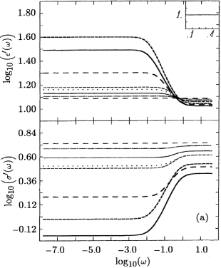
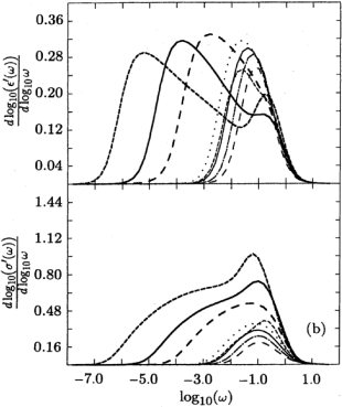
[70.2.2.4] Figure 2 presents the uniformly connected model with
are presented.
[70.2.2.4] Figure 2 presents the uniformly connected model with ![]() ,
Figure 3 the uniformly connected model with
,
Figure 3 the uniformly connected model with ![]() .
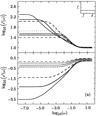
[70.2.2.5] Figure 4 gives the results
for the central pore model with
.
[70.2.2.5] Figure 4 gives the results
for the central pore model with
![]() ,
and Fig. 5 those
for the grain consolidation model with
,
and Fig. 5 those
for the grain consolidation model with
![]() .
[70.2.2.6] In each figure the line styles correspond to the line styles
of the local porosity distributions displayed in Figure 1.
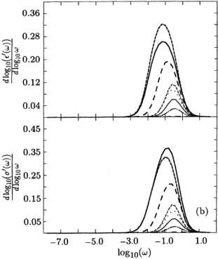
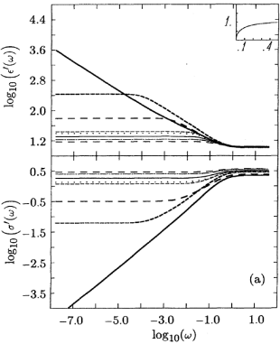
[70.2.2.7] Parts (a) of each figure shows
.
[70.2.2.6] In each figure the line styles correspond to the line styles
of the local porosity distributions displayed in Figure 1.
[70.2.2.7] Parts (a) of each figure shows ![]() as a function of
as a function of ![]() in the upper graph and
in the upper graph and ![]() in the lower graph.
[70.2.2.8] In addition, the inset in the upper right-hand corner
displays the local percolation
probability
in the lower graph.
[70.2.2.8] In addition, the inset in the upper right-hand corner
displays the local percolation
probability ![]() for
for ![]() .
[70.2.2.9] The vertical scale for the inset is always
.
[70.2.2.9] The vertical scale for the inset is always ![]() .
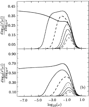
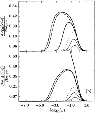
[70.2.2.10] Part (b) display in the upper graph
.
[70.2.2.10] Part (b) display in the upper graph ![]() versus
versus ![]() and
and ![]() in the lower plot.
[70.2.2.11] These quantities give a more sensitive
representation of the dispersion
and show at the same time the values
of “local exponents”.
[70.2.2.12] In all figures frequency is measured in units
of the relaxation frequency
of water as discussed in Section IV.
[70.2.2.13] All plots are given over ten frequency
decades with a resolution of five points per decade.
in the lower plot.
[70.2.2.11] These quantities give a more sensitive
representation of the dispersion
and show at the same time the values
of “local exponents”.
[70.2.2.12] In all figures frequency is measured in units
of the relaxation frequency
of water as discussed in Section IV.
[70.2.2.13] All plots are given over ten frequency
decades with a resolution of five points per decade.
 |
 |
 |
 |
 |
 |
 |
 |
E Discussion
[70.2.3.1] It is obvious from Figs. 2-5 [especially part (b)]
that the low-frequency dielectric response
depends sensitively on the details of ![]() and
and ![]() .
[70.2.3.2] A general discussion is difficult,
because the response is always a mixture
between three basic mechanisms each of which can give
significant dielectric dispersion.
[page 71, §0]
[71.1.0.1] The first mechanism is the dispersion
resulting from the disorder in
.
[70.2.3.2] A general discussion is difficult,
because the response is always a mixture
between three basic mechanisms each of which can give
significant dielectric dispersion.
[page 71, §0]
[71.1.0.1] The first mechanism is the dispersion
resulting from the disorder in ![]() itself.
[71.1.0.2] The second mechanism is the despersion resulting from
itself.
[71.1.0.2] The second mechanism is the despersion resulting from ![]() ,
i.e., from percolation geometry.
[71.1.0.3] The third mechanism is the dispersion
resulting from the behavior of
,
i.e., from percolation geometry.
[71.1.0.3] The third mechanism is the dispersion
resulting from the behavior of ![]() in the
in the ![]() limit, i.e., the thin-plate effect.
limit, i.e., the thin-plate effect.
[71.1.1.1] The absolute dispersion for all figures is collected
in Table 2.
[71.1.1.2] ![]() is defined as
is defined as ![]() ,
while
,
while ![]() .
.
[71.2.1.1] Before discussing the three mechanisms,
it is important to note that the bulk porosity ![]() does not influence the shape of the response curves
if it is changed without changing the shape of
does not influence the shape of the response curves
if it is changed without changing the shape of ![]() .
[71.2.1.2] Instead, it determines an overall frequency shift
for the frequency region over which the dispersion occurs.
[71.2.1.3] As
.
[71.2.1.2] Instead, it determines an overall frequency shift
for the frequency region over which the dispersion occurs.
[71.2.1.3] As ![]() is lowered,
this region is shifted toward lower frequencies.
[71.2.1.4] This observation together with the fact
that all
is lowered,
this region is shifted toward lower frequencies.
[71.2.1.4] This observation together with the fact
that all ![]() give the same bulk
porosity of
give the same bulk
porosity of
![]() shows
that the bulk porosity by itself cannot be used
to characterize the dielectric response.
[71.2.1.5] In particular, there is no theoretical basis
for Archie’s law [eq. (5.27)]
if interpreted as a relation between
dc conductivity and bulk porosity
(see Section V.D for a discussion).
shows
that the bulk porosity by itself cannot be used
to characterize the dielectric response.
[71.2.1.5] In particular, there is no theoretical basis
for Archie’s law [eq. (5.27)]
if interpreted as a relation between
dc conductivity and bulk porosity
(see Section V.D for a discussion).
[page 72, §0]
[page 73, §0]
[73.1.1.1] A second observation is that in all figures
the high-frequency real dielectric constant ![]() is not very sensitive to the details of
is not very sensitive to the details of ![]() .
[73.1.1.2] This is a consequence of the fact
that for low
.
[73.1.1.2] This is a consequence of the fact
that for low ![]() the local dielectric constants
the local dielectric constants ![]() and
and ![]() must both approach
must both approach ![]() .
.
[73.1.2.1] The first mechanism, dispersion from the form of ![]() ,
can be studied in pure form when
,
can be studied in pure form when ![]() ,
and the corresponding results are shown in Figure 2.
[73.1.2.2] In this case there are no blocking local geometries;
i.e.,
,
and the corresponding results are shown in Figure 2.
[73.1.2.2] In this case there are no blocking local geometries;
i.e., ![]() according to eq. (5.7).
[73.1.2.3] If
according to eq. (5.7).
[73.1.2.3] If ![]() is highly peaked as in curve 2,
then the system is only weakly disordered,
and there is almost no visible disperion
with the amount of disorder
contained in
is highly peaked as in curve 2,
then the system is only weakly disordered,
and there is almost no visible disperion
with the amount of disorder
contained in ![]() .
[73.1.2.4] In fact, distributions with power-law
divergences at
.
[73.1.2.4] In fact, distributions with power-law
divergences at ![]() or with percolation structure
generate the strongest dispersion,
as can be seen from curves 3 and 5-8 in figure 2.
[73.1.2.5] Table 2 shows that the dispersion
varies almost three orders of magnitude
between the different distributions.
[73.1.2.6] Note that relatively similar
local porosity distributions
such as curves 6 and 8
can have very different dielectric response.
[73.1.2.7] On the other hand, very different shapes
for
or with percolation structure
generate the strongest dispersion,
as can be seen from curves 3 and 5-8 in figure 2.
[73.1.2.5] Table 2 shows that the dispersion
varies almost three orders of magnitude
between the different distributions.
[73.1.2.6] Note that relatively similar
local porosity distributions
such as curves 6 and 8
can have very different dielectric response.
[73.1.2.7] On the other hand, very different shapes
for ![]() can give similar
can give similar ![]() ,
as demonstrated by curves 3 and 5.
[73.1.2.8] This shows that the dielectric response by itself
does not contain a full geometric characterization
of the pore space,
and it needs always to be complemented
with additional physical or geometrical information.
[73.1.2.9] This is not too surprising.
[73.1.2.10] Indeed, it is more surprising
that when the dielectric response becomes large
it is also very sensitive to geometric details.
[73.1.2.11] This is the case for dielectric enhancement
near the percolation threshold
or as a result of the thin-plate effect.
,
as demonstrated by curves 3 and 5.
[73.1.2.8] This shows that the dielectric response by itself
does not contain a full geometric characterization
of the pore space,
and it needs always to be complemented
with additional physical or geometrical information.
[73.1.2.9] This is not too surprising.
[73.1.2.10] Indeed, it is more surprising
that when the dielectric response becomes large
it is also very sensitive to geometric details.
[73.1.2.11] This is the case for dielectric enhancement
near the percolation threshold
or as a result of the thin-plate effect.
[73.1.3.1] Consider the thin-plate mechanism.
[73.1.3.2] It requires the presence of blocking geometries
of high porosity.
[73.1.3.3] Mathematically, this means ![]() for large
for large ![]() .
[73.1.3.4] As a simple illustration, Figure 3 displays the results
for the uniformly connected model
when
.
[73.1.3.4] As a simple illustration, Figure 3 displays the results
for the uniformly connected model
when ![]() .
[73.1.3.5] Now
.
[73.1.3.5] Now ![]() , which is far away from
, which is far away from ![]() .
[73.1.3.6] Nevertheless, the dielectric dispersion
is much stronger than would be obtained
for solutions to the central pore model
or grain consolidation model with the same
.
[73.1.3.6] Nevertheless, the dielectric dispersion
is much stronger than would be obtained
for solutions to the central pore model
or grain consolidation model with the same ![]() .
[73.1.3.7] Compare, e.g., curve 5 in figure 3
with curve 5 in figure 5.
[73.1.3.8] Moreover, the dielectric dispersion
becomes sensitive to the details
.
[73.1.3.7] Compare, e.g., curve 5 in figure 3
with curve 5 in figure 5.
[73.1.3.8] Moreover, the dielectric dispersion
becomes sensitive to the details ![]() .
[73.1.3.9] It is now possible to distinguish in figure 3(b)
the distributions 3, 7 and 8,
which have
.
[73.1.3.9] It is now possible to distinguish in figure 3(b)
the distributions 3, 7 and 8,
which have ![]() from the rest for which
from the rest for which ![]() .
[73.1.3.10] In particular, curves 3 and 5,
which had very similar response in figure 2,
appear now very different.
[73.1.3.11] The dispersion is the stronger
the more weight
.
[73.1.3.10] In particular, curves 3 and 5,
which had very similar response in figure 2,
appear now very different.
[73.1.3.11] The dispersion is the stronger
the more weight ![]() has at high
has at high ![]() .
[73.1.3.12] This can be seen from curve 3,
which shows less dispersion than curves 4 and 5,
while the opposite was true for figure 2.
[73.2.0.1] Similarly,
.
[73.1.3.12] This can be seen from curve 3,
which shows less dispersion than curves 4 and 5,
while the opposite was true for figure 2.
[73.2.0.1] Similarly, ![]() for curve 7
is depressed below curves 6 and 8 at intermediate frequencies.
[73.2.0.2] At very low frequencies,
the percolative character of distribution 7
is responsible for stronger overall dispersion
than in curve 6.
[73.2.0.3] The degree of asymmetry of
for curve 7
is depressed below curves 6 and 8 at intermediate frequencies.
[73.2.0.2] At very low frequencies,
the percolative character of distribution 7
is responsible for stronger overall dispersion
than in curve 6.
[73.2.0.3] The degree of asymmetry of ![]() is reflected in the asymmetry of the response,
as best seen in the derivatives plotted in figure 3(b).
is reflected in the asymmetry of the response,
as best seen in the derivatives plotted in figure 3(b).
[73.2.1.1] The percolation mechanism is responsible
for strong dielectric disperion
in figures 4 and 5.
[73.2.1.2] There is essentially no dispersion
from thin-plate mechanism in these cases
because in both cases ![]() for
for
![]() ,
and thus there are no local geometrics with
a high dielectric constant.
[73.2.1.3] Figure 4 represents the central
pore model with
,
and thus there are no local geometrics with
a high dielectric constant.
[73.2.1.3] Figure 4 represents the central
pore model with
![]() ,
and results for the grain consolidation model
with
,
and results for the grain consolidation model
with
![]() are given in figure 5.
[73.2.1.4] Contrary to the situation in figures 2 and 3,
are given in figure 5.
[73.2.1.4] Contrary to the situation in figures 2 and 3,
![]() is now different for each distribution.
[73.2.1.5] The results of performing the integral
in eq. (5.7) are listed in table 3.
[73.2.1.6] Naturally, the dielectric dispersion
increases strongly with
is now different for each distribution.
[73.2.1.5] The results of performing the integral
in eq. (5.7) are listed in table 3.
[73.2.1.6] Naturally, the dielectric dispersion
increases strongly with ![]() and this effect dominates the dispersion from
and this effect dominates the dispersion from ![]() itself.
[73.2.1.7] In particular, for
itself.
[73.2.1.7] In particular, for ![]() power-law behavior for
power-law behavior for ![]() as a function of frequency is obtained
in agreement with the scaling theory
presented in Section V.
[73.2.1.8] As an example, scaling theory
predicts the exponent
as a function of frequency is obtained
in agreement with the scaling theory
presented in Section V.
[73.2.1.8] As an example, scaling theory
predicts the exponent
![]() for the conductivity of distribution 8 in figure 4 and
for the conductivity of distribution 8 in figure 4 and
![]() for the real dielectric constants.
[73.2.1.9] These predictions are obtained
from eqs. (5.23) and (5.24)
using
for the real dielectric constants.
[73.2.1.9] These predictions are obtained
from eqs. (5.23) and (5.24)
using ![]() and eqs. (5.13b)
and (6.12) with
and eqs. (5.13b)
and (6.12) with
![]() ,
and the exponent
,
and the exponent ![]() from Table 1.
[73.2.1.10] Figure 4(b) shows that these values
are indeed approached at low frequencies.
[73.2.1.11] Similarly, scaling theory predicts the exponent
from Table 1.
[73.2.1.10] Figure 4(b) shows that these values
are indeed approached at low frequencies.
[73.2.1.11] Similarly, scaling theory predicts the exponent ![]() for
for ![]() and
and ![]() corresponding
to distributions
corresponding
to distributions ![]() ,
, ![]() and
and ![]() in figure 5.
[73.2.1.12] Again, these values are approached
as seen fom figure 5(b),
although the power-law behavior
occurs over a limited frequency range
because
in figure 5.
[73.2.1.12] Again, these values are approached
as seen fom figure 5(b),
although the power-law behavior
occurs over a limited frequency range
because ![]() is not sufficiently
close to the critical region.
[73.2.1.13] Note that curve 8 in figure 5
has dropped below the percolation threshold,
and thus the conductivity increases as
is not sufficiently
close to the critical region.
[73.2.1.13] Note that curve 8 in figure 5
has dropped below the percolation threshold,
and thus the conductivity increases as ![]() for small
for small ![]() .
.
| Curve No. 1 | 1 | 2 | 3 | 4 | 5 | 6 | 7 | 8 |
|---|---|---|---|---|---|---|---|---|
|
|
0.798 | 0.053 | 3.716 | 1.863 | 3.147 | 9.261 | 28.793 | 20.484 |
|
|
0.298 | 0.035 | 1.067 | 0.619 | 0.889 | 1.545 | 2.400 | 2.029 |
|
|
19.197 | 13.819 | 21.956 | 25.162 | 34.950 | 96.046 | 186.010 | 115.270 |
|
|
1.585 | 1.370 | 1.664 | 1.674 | 1.741 | 1.648 | 1.751 | 1.489 |
|
|
5.996 | 3.835 | 16.616 | 9.639 | 14.204 | 52.196 | 259.700 | 3932.522 |
|
|
1.105 | 0.801 | 1.974 | 1.455 | 1.708 | 2.176 | 2.877 | 2.283 |
|
|
2.119 | 0.053 | 371.525 | 5.498 | 11.430 | 291.481 | 277.396 | 37.691 |
|
|
0.595 | 0.035 | 3.025 | 1.137 | 1.604 | 2.565 | 3.043 | 2.436 |
[73.2.2.1] The complexity and variability of ![]() obtained from the simple mean-field solutions
of this section correspond to the complexity
and variability of possible pore-space geometries.
[73.2.2.2] More approximate analytical investigations
of the solutions to eq. (3.2)
are necessary to identify simple parameters
characterizing
obtained from the simple mean-field solutions
of this section correspond to the complexity
and variability of possible pore-space geometries.
[73.2.2.2] More approximate analytical investigations
of the solutions to eq. (3.2)
are necessary to identify simple parameters
characterizing ![]() and
and ![]() which allow a better classification
of the solutions and thereby the possible geometries.
which allow a better classification
of the solutions and thereby the possible geometries.
| Curve No. | 1 | 2 | 3 | 4 | 5 | 6 | 7 | 8 |
|---|---|---|---|---|---|---|---|---|
| CPM | 0.6542 | 0.6940 | 0.5420 | 0.5858 | 0.5341 | 0.4059 | 0.3643 | 0.3334 |
| GCM | 0.7500 | 1.0000 | 0.3399 | 0.6048 | 0.4962 | 0.3415 | 0.3376 | 0.2841 |
F Sedimentary rock
[73.2.3.1] The present paper deals only
with simple homogeneous and isotropic porous media.
[73.2.3.2] Real rocks are highly inhomogeneous,
but they can also be discussed
within the present framework.
[page 74, §0]
[74.1.0.1] Sedimentary rocks exhibit two main types of porosity.
[74.1.0.2] Primary interparticle porosity
is the porosity between the grains
of the original sediment.
[74.1.0.3] Often, this pore space is changed
during diagenesis of the sediment.
[74.1.0.4] In particular cements between the grains
can exhibit a qualitatively different secondary porosity.[33]
[74.1.0.5] This situation can be treated within
the present formalism
by replacing the dielectric constant ![]() of the pore-filling fluid
with the effective dielectric constant
of the pore-filling cement.
[74.1.0.6] Naturally, the results must be much more complex,
as they contain additional
independent geometrical information describing the cement.
of the pore-filling fluid
with the effective dielectric constant
of the pore-filling cement.
[74.1.0.6] Naturally, the results must be much more complex,
as they contain additional
independent geometrical information describing the cement.
