2 Relation between fractional and fractal walks
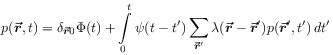
[1.3.3.1] Let us start by recalling briefly the general theory of continuous time random walks [5, 7, 8]. [1.3.3.2] The basic equation of motion is the continous time random walk (CTRW) integral equation [16]
 |
(2.1) |
[page 2, §0]
describing a random walk in continous time without correlation
between its spatial and temporal behaviour.
[2.1.0.1] Here, as in (1.2),
![]() denotes the probability density to find the diffusing
entity at the position
denotes the probability density to find the diffusing
entity at the position ![]() at time
at time ![]() if it started from
the origin
if it started from
the origin ![]() at time
at time ![]() .
[2.1.0.2]
.
[2.1.0.2] ![]() is the probability
for a displacement
is the probability
for a displacement ![]() in each single step, and
in each single step, and ![]() is the
waiting time distribution giving the probability density
for the time interval
is the
waiting time distribution giving the probability density
for the time interval ![]() between two consecutive steps.
[2.1.0.3] The transition probabilities obey
between two consecutive steps.
[2.1.0.3] The transition probabilities obey ![]() .
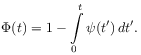
[2.1.0.4] The function
.
[2.1.0.4] The function ![]() is the survival probability at the initial
position which is related to the waiting time distribution through
is the survival probability at the initial
position which is related to the waiting time distribution through
 |
(2.2) |
[2.1.0.5] The objective of this paper which was defined in the introduction is to show that the fractional master equation (1.2) is a special case of the CTRW-equation (2.1), and to find the appropriate waiting time density.
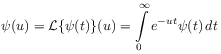
[2.1.1.1] The translation invariant form of the transition probabilities in (2.1) allows a solution through Fourier-Laplace transformation. [2.1.1.2] Let
 |
(2.3) |
denote the Laplace transform of ![]() and
and
| (2.4) |
the Fourier transform of ![]() , which is also called
the structure function of the random walk [5].
[2.1.1.3] Then the
Fourier Laplace transform
, which is also called
the structure function of the random walk [5].
[2.1.1.3] Then the
Fourier Laplace transform ![]() of the solution to (2.1)
is given as [5, 7, 8, 16]
of the solution to (2.1)
is given as [5, 7, 8, 16]
| (2.5) |
where ![]() is the Laplace transform of the survival probability.
is the Laplace transform of the survival probability.
[2.1.2.1] Similarly the fractional master equation (1.2) can be solved in Fourier-Laplace space with the result
| (2.6) |
where ![]() is the Fourier transform of the kernel
is the Fourier transform of the kernel ![]() in (1.2).
[2.1.2.2] Eliminating
in (1.2).
[2.1.2.2] Eliminating ![]() between (2.5) and
(2.6) gives the result
between (2.5) and
(2.6) gives the result
| (2.7) |
where ![]() is a constant.
[2.1.2.3] The last equality obtains because the
left hand side of the first equality is
is a constant.
[2.1.2.3] The last equality obtains because the
left hand side of the first equality is ![]() -independent while
the right hand side is independent of
-independent while
the right hand side is independent of ![]() .
.
[2.1.3.1] From (2.7) it is seen that the fractional
master equation characterized by the kernel ![]() and the
order
and the
order ![]() corresponds to a special class of space time
decoupled continuous time random walks characterized by
corresponds to a special class of space time
decoupled continuous time random walks characterized by
![]() and
and ![]() .
[2.1.3.2] This correspondence is given precisely as
.
[2.1.3.2] This correspondence is given precisely as
| (2.8) |
and
| (2.9) |
with the same constant ![]() appearing in both equations.
[2.2.0.1] Not unexpectedly the correspondence defines the waiting
time distribution uniquely up to a constant while the
structure function is related to the Fourier transform
of the transition rates.
appearing in both equations.
[2.2.0.1] Not unexpectedly the correspondence defines the waiting
time distribution uniquely up to a constant while the
structure function is related to the Fourier transform
of the transition rates.
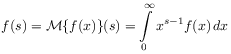
[2.2.1.1] To invert the Laplace transformation in (2.8)
and exhibit the form of the waiting time density ![]() in the time domain it is convenient to introduce the
Mellin transformation
in the time domain it is convenient to introduce the
Mellin transformation
 |
(2.10) |
for a function ![]() .
[2.2.1.2] The Mellin transformed waiting time
density is obtained as
.
[2.2.1.2] The Mellin transformed waiting time
density is obtained as
| (2.11) |
where ![]() denotes the Gamma function.
[2.2.1.3] To obtain (2.11)
from (2.8) the relation between Laplace and Mellin transforms
denotes the Gamma function.
[2.2.1.3] To obtain (2.11)
from (2.8) the relation between Laplace and Mellin transforms
| (2.12) |
the special result
| (2.13) |
and the general relation
| (2.14) |
valid for ![]() have been employed.
[2.2.1.4] Using the definition of the general
have been employed.
[2.2.1.4] Using the definition of the general ![]() -function given in the
appendix one obtains the result
-function given in the
appendix one obtains the result
| (2.15) |
which may be rewritten as
| (2.16) |
with the help of general relations for ![]() -functions [24].
[2.2.1.5] The dependence on the parameters
-functions [24].
[2.2.1.5] The dependence on the parameters ![]() and
and ![]() has been indicated
explicitly.
[2.2.1.6] From the series expansion of
has been indicated
explicitly.
[2.2.1.6] From the series expansion of ![]() -functions given in the appendix
one finds
-functions given in the appendix
one finds
[page 3, §0]
| (2.17) |
showing that ![]() behaves as
behaves as
| (2.18) |
for small ![]() .
[3.1.0.1] Because
.
[3.1.0.1] Because ![]() the waiting time density
is singular at the origin.
[3.1.0.2] The series representation (2.17)
shows that the waiting time density is a natural generalization of an
exponential waiting time density to which it reduces for
the waiting time density
is singular at the origin.
[3.1.0.2] The series representation (2.17)
shows that the waiting time density is a natural generalization of an
exponential waiting time density to which it reduces for ![]() ,
i.e.
,
i.e. ![]() .
[3.1.0.3] The series in (2.17) is recognized as the generalized
Mittag-Leffler function
.
[3.1.0.3] The series in (2.17) is recognized as the generalized
Mittag-Leffler function ![]() [25], and
[25], and ![]() may thus be written alternatively as
may thus be written alternatively as
| (2.19) |
[3.1.0.4] Of course the result (2.17) can also be obtained more directly, but we have presented here a method using Mellin transforms because it remains applicable in cases where a direct inversion fails [23]. [3.1.0.5] The asymptotic expansion of the Mittag-Leffler function for large argument [25] yields
| (2.20) |
for large ![]() and
and ![]() .
[3.1.0.6] This result shows that the waiting time
distribution has an algebraic tail of the kind usually considered
in the theory of random walks [12, 13, 14, 15, 16].
.
[3.1.0.6] This result shows that the waiting time
distribution has an algebraic tail of the kind usually considered
in the theory of random walks [12, 13, 14, 15, 16].
