Article

[page 1, §1]
[1.1.1.1] Accurate prediction and understanding of material parameters for disordered systems such as rocks [1], soils [2], papers [3], clays [4], ceramics [5], composites [6], microemulsions [7] or complex fluids require geometrical microstructures as a starting point as emphasized by Landauer [8] and numerous authors [9, 10, 11, 12]. [1.1.1.2] Digital three dimensional images of unprecedented size and accuracy have been prepared for the case of Fontainebleau sandstone, and are being made available to the scientific community in this brief report.

[1.1.2.1] Multiscale modelling of disordered media has recently become a research focus in mathematics and physics of complex materials and porous media [13, 14, 15, 16, 17, 18]. [1.1.2.2] Accurate prediction of physical observables for multiscale heterogeneous media is a perennial problem [9, 8]. [1.1.2.3] It requires knowledge of the three dimensional disordered microstructure [11]. [1.1.2.4] Our objective in this brief report is to provide to the scientific public a sequence of fully three dimensional digital images with a realistic strongly correlated microstructure typical for sandstone. [1.1.2.5] Resolutions from $a=117.18\mu m$ to $0.4576\mu m$ are available for download [19]. [1.1.2.6] Experimental computed microtomographic images of comparable size, resolution or data quality are, to the best of our knowledge, not available at present. [1.1.2.7] More importantly, experimental images of similar size and quality are not expected to become available to the scientific community in the near future.

[1.1.3.1] Despite the impressive progress in fully three dimensional high resolution X-ray and synchrotron computed tomography of porous media in recent years [20, 21] acquisition times for 1500 radiograms needed for a $1024\times 1024\times 1024$ -sample of average quality at the ID19 beamline of the European Synchrostron Radiation Facility are on the order of 30 minutes [22]. [1.1.3.2] Extrapolating to the number of 32768 such blocks, that we provide in this report, would thus require on the order of 16384 hours or roughly 2 years of uninterrupted beamtime. [1.1.3.3] It is unlikely that this amount of beamtime will ever be spent.

[1.1.4.1] The continuum multiscale modeling technology for carbonates developed in [23, 24, 25] was applied to Fontainebleau sandstone in [26], to create a synthetic, non-experimental image at very high resolution. [1.2.0.1] A laboratory sized cubic sample of sidelength $1.8$ cm was generated containing roughly $1.02\times 10^{6}$ polyhedral quartz grains. [1.2.0.2] For simplicity there are a total of 99 grain types each defined by eighteen intersecting planes. [1.2.0.3] The grains are rescaled, randomly oriented and have a prescribed overlap with each other (see [26] for more modeling details). [1.2.0.4] The model was geometrically calibrated against a well studied experimental microtomogram at $7.5\mu m$ resolution [27]. [1.2.0.5] The geometric calibration was based on matching porosity, specific surface, integrated mean curvature, Gaussian curvature, correlation function, local porosity distributions (with $240\mu m$ and $480\mu m$ measurement cell size), and local percolation probabilities at the same measurement cell sizes. [1.2.0.6] Comparison of these quantities at $a=7.5\mu m$ was carried out in [26].

[1.2.1.1] The continuum sample generated and characterized in [26] is the starting point for the work reported here. [1.2.1.2] To eliminate boundary effects a centered cubic sample, denoted by $\mathbb{S}$ , of sidelength $1.5$ cm was cropped from the original deposit. [1.2.1.3] The pore space inside $\mathbb{S}$ is denoted by $\mathbb{P}$ , the matrix region is denoted $\mathbb{M}$ .

[1.2.2.1] The sample region $\mathbb{S}$ was discretized into $N$ cubic voxels $\mathbb{V}_{i}(a)\subset\mathbb{S}$ $(i=1,\dots,N$ ), whose sidelength $a$ is a multiple of the base resolution $a_{0}=1.5\text{cm}/16384=0.9155273\mu m$ . [1.2.2.2] The discretization employs a cubic array of $6^{3}=216$ collocation points placed centrally and distributed uniformly inside each voxel $\mathbb{V}_{i}(a)$ . [1.2.2.3] It yields an integer gray scale value $0\leq g_{i}(a)\leq 216$ with $1\leq i\leq N$ for each of the $N$ voxels (discrete [page 2, §0] volume elements). [2.1.0.1] The gray value $g_{i}(a)\in\mathbb{N}$ equals the number of collocation points inside voxel $\mathbb{V}_{i}$ , that fall into the matrix region $\mathbb{M}$ [26]. The gray values approximate the integral

$\psi _{i}(a)=\frac{1}{a^{3}}\int\limits _{{\mathbb{V}_{i}\cap\mathbb{P}}}\textrm{d}^{3}x\approx 1-\frac{g_{i}(a)}{216},$

(1)

which is the porosity inside the voxel $\mathbb{V}_{i}$ at resolution $a$ . [2.1.0.2] Thus, $g_{i}(a)=0$ approximates $\mathbb{V}_{i}\subset\mathbb{P}$ , while $g_{i}(a)=216$ approximates $\mathbb{V}_{i}\subset\mathbb{M}$ .

$a$	$128a_{0}$	$64a_{0}$	$32a_{0}$	$16a_{0}$	$8a_{0}$	$4a_{0}$	$2a_{0}$	$a_{0}$	$a_{0}/2$
$L$	128	256	512	1024	2048	4096	8192	16384	32768
$N$	$2^{{21}}$	$2^{{24}}$	$2^{{27}}$	$2^{{30}}$	$2^{{33}}$	$2^{{36}}$	$2^{{39}}$	$2^{{42}}$	$2^{{45}}$
$K$	1	1	1	1	8	64	512	4096	32768
$T_{{\rm CPU}}$ [h]	1.6	3.2	6.5	11	88	704	5632	45056	360448

Table 1: Overview of data sets available from http:www.icp.uni-stuttgart.demicroct for download. $a$ is the resolution in units of $a_{0}=0.91552734\mu m$ . $L$ is the sidelength of the cubic sample in units of $aa_{0}$ . The total number of voxels is $N$ , and $K$ is the number of cubic blocks used to represent the sample. One has $K>1$ whenever $L>1024$ . $T_{{\rm CPU}}$ gives an estimate of the total CPU time in hours, that was used to generate the discretizations. Calculations were typically performed in parallel on 512 Xeon processors requiring a total wall time of approximately $T_{{\rm wall}}=T_{{\rm CPU}}/512$ in hours due to an essentially linear speedup. Total wall time was around 800 hours or 34 days.

[2.1.1.1] At the lowest resolution $a=128a_{0}=117.18\mu m$ the sample consists of $N=128\times 128\times 128=2~097~152$ discrete volume elements (voxels), and it can easily be stored in a single file. [2.1.1.2] At higher resolution this becomes technically inconvenient, and we have limited the file size to blocks with $1024\times 1024\times 1024=1~073~741~824$ voxels corresponding to roughly 1 Gigabyte. [2.1.1.3] The highest resolution at which the sample is still stored in a single file is $a=16a_{0}=14.65\mu m$ . [2.1.1.4] For resolutions $a\leq 8a_{0}=7.3244\mu m$ the data are stored in several blocks. [2.1.1.5] This results in a maximum of 32768 blocks for the highest resolution of $a=a_{0}/2=0.4576\mu m$ . [2.1.1.6] The number of voxels is $N=2^{{45}}=35~184~372~088~832$ at this resolution. [2.1.1.7] Table 1 gives a summary of the available resolutions $a$ , sample sidelength $L$ (in units of $a$ ), number of voxels $N$ , number of $1024^{3}$ -blocks $K$ , and an estimate of the CPU time and wall time expended for the computation.

[2.1.2.1] All computations were performed on the HLRS’s bwGRID cluster at the Universität Stuttgart consisting of 498 compute nodes each holding two Intel Xeon CPU’s capable of 11.32 GFLOPs. [2.1.2.2] The peak performance (Linpack) is 38 TFLOP [28]. For the calculations performed in this work 256 nodes (=512 CPU’s) were used in parallel. [2.1.2.3] The discretization algorithm was parallelized, but not optimized. [2.1.2.4] Every discretized volume element (voxel) requires one byte of storage. [2.1.2.5] The storage requirements without compression amount to roughly 40 Terabytes.

[2.1.3.1] The results can be used to calculate resolution dependent geometric and physical properties. [2.1.3.2] Because the underlying continuum microstructure is available with floating point precision, the resolution can be changed over many decades. [2.1.3.3] Resolution dependent geometrical or physical properties can be compared with, or extrapolated to, the continuum result. [2.1.3.4] This is illustrated with the porosity $\phi$ (volume fraction of pore space) and specific internal surface $S$ (surface area per unit volume).

[2.1.4.1] The exact values of $\phi$ and $S$ are not known for the continuum model. [2.1.4.2] Depending on the geometrical or physical quantity of interest computations on the continuum model as well as computations on discretizations with more than $1024^{3}$ discrete volume elements are (as a rule) challenging at present.

[2.1.5.1] The discretized samples approximate the exact geometry of the continuum model. [2.1.5.2] Let $\delta _{{ij}}=1$ for $i=j$ and $\delta _{{ij}}=0$ for $i\neq j$ . [2.2.0.1] Then

$M(g,a)=\sum _{{i=1}}^{N}\delta _{{gg_{i}(a)}}$

(2)

is the number of voxels with grey value $g$ at resolution $a$ , and

$\phi({g_{{\rm th}}},a)=\frac{1}{N}\sum _{{g=0}}^{{g_{{\rm th}}}}M(g,a)$

(3)

is an estimate for the porosity based on a segmentation of its discretization at resolution $a$ with segmentation threshold ${g_{{\rm th}}}$ . [2.2.0.2] The porosity $\phi=\lim _{{a\to 0}}\phi({g_{{\rm th}}},a)$ of the continuum model at infinite resolution is expected to obey

$\phi(0,a)\leq\phi\leq\phi(215,a)$

(4)

for all ${g_{{\rm th}}}$ and all $a$ . [2.2.0.3] The validity of these bounds depends on the continuum microstructure. [2.2.0.4] They are expected to hold approximately for the sandstone microstructure. [2.2.0.5] Grey values $g=0$ and $g=216$ do not guarantee, that the pore boundary does not intersect the voxel region, although it will be true for the majority of voxels in the limit $a\to 0$ .

Figure 1: Porosity $\phi({g_{{\rm th}}},a)$ as function of segmentation threshold ${g_{{\rm th}}}$ for resolutions $a=8a_{0},4a_{0},2a_{0},a_{0},a_{0}/2$ .

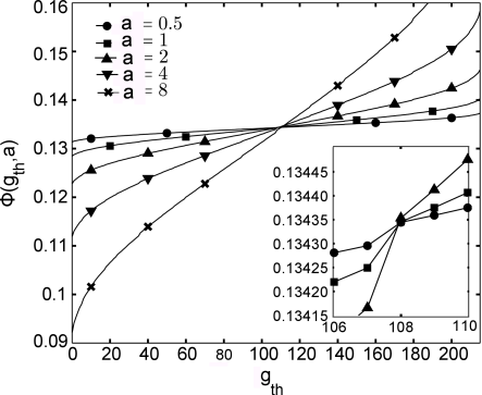
[2.2.1.1] Figure 1 shows the porosity $\phi({g_{{\rm th}}},a)$ as a function of the segmentation threshold ${g_{{\rm th}}}$ for resolutions $a=8a_{0},4a_{0},2a_{0},a_{0},a_{0}/2$ .

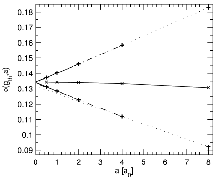
[2.2.2.1] Figure 2 shows the porosity bounds $\phi(0,a)$ and $\phi(215,a)$ for resolutions $a=8a_{0},4a_{0},2a_{0},a_{0},a_{0}/2$ . [2.2.2.2] It also shows eight extrapolations defined as the linear functions

$\phi _{i}(a;c)=\varphi _{i}(c)+k_{i}(c)a$

(5)

where $i\in\{ 0,215\}$ and the slopes $k_{i}(c)$ and intercepts $\varphi _{i}(c)$ are determined such that

$\phi _{i}(a;c)=\phi(i,a)$

(6)

for $a=c$ and $a=c/2$ . [2.2.2.3] Table 2 lists the slopes and intercepts of all eight extrapolations. [2.2.2.4] In between the upper and lower bounds Figure 2 also shows (with symbols $\times$ connected by a solid line) the porosity obtained by maximizing the variance [page 3, §0] of the grey scale histogram, a standard technique in image processing [29].

$c$	$k_{0}(c)$	$\varphi _{0}(c)$	$k_{{215}}(c)$	$\varphi _{{215}}(c)$
$8a_{0}$	-0.004944104133756	0.131677153054625	0.006128869055829	0.133806445926894
$4a_{0}$	-0.005437994277600	0.133652713629999	0.006038194581379	0.13416914382469
$2a_{0}$	-0.005680456774371	0.134137638623542	0.005981708264244	0.134282116458962
$a_{0}$	-0.005843877976029	0.134301059825200	0.005942813391024	0.13432101133218

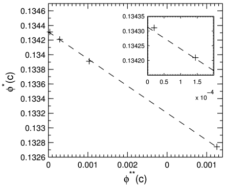
Table 2: Slopes and intercepts for extrapolations in Figure 2 according to equation (5).

[3.1.1.1] Figure 3 shows the mean values

$\phi^{*}(c)=\frac{\varphi _{0}(c)+\varphi _{{215}}(c)}{2}$

(7)

plotted against the differences

$\phi^{{**}}(c)=\varphi _{{215}}(c)-\varphi _{0}(c)$

(8)

as data points. [3.1.1.2] It also shows a linear fit to the data as a dashed line. [3.1.1.3] The linear fit extrapolates to the value

$\lim _{{c\to 0}}\phi^{*}(c)=0.134313\pm 0.00001$

(9)

where the uncertainty is from the residues of the fit.

Figure 2: Approximate lower bounds $\phi(0,a)$ and approximate upper bounds $\phi(215,a)$ for the porosity $\phi$ for resolutions $a=8a_{0},4a_{0},2a_{0},a_{0},a_{0}/2$ are shown as (+) data points. A total of eight straight lines show extrapolations of these upper and lower bounds to $a=0$ . The symbols $\times$ connected by a solid line show the porosity estimated from maximizing the variance of the grey scale histogram.

Figure 3: Linear fit to the mean values $\phi^{*}(c)$ versus differences $\phi^{{**}}(c)$ for $c=8a_{0},4a_{0},2a_{0},a_{0}$ .

$a[a_{{0}}]$	8	4	2	1	0.5
$S_{{\rm max}}(a)$ [mm ${}^{{-1}}$ ]	20.039	20.530	20.774	20.904	20.946
$S_{{\rm mf}}(a)$ [mm ${}^{{-1}}$ ]	9.6371	9.8774	9.9978	10.061	10.065
$S_{{\rm min}}(a)$ [mm ${}^{{-1}}$ ]	6.0407	6.1915	6.2673	6.3068	6.3096
$S_{{\rm measured}}(a)$ [mm ${}^{{-1}}$ ]	9.168 $\pm$ 0.02	9.825 $\pm$ 0.06	10.159 $\pm$ 0.16	$10.307(\pm 0.43)$	10.355 $(\pm 1.34)$

Table 3: $S_{{\rm max}}(a)$ and $S_{{\rm min}}(a)$ are the upper and lower bounds computed from eqs. (16) resp. (17) and eq. (18) for specific internal surfaces as functions of resolution $a$ . $S_{{\rm mf}}(a)$ is the mean field estimate computed from eqs. (18)–(23). $S_{{\rm measured}}(a)$ is calculated by applying the direct algorithm from [30] to thresholded cubic subsamples, and averaging the results as described in the last paragraph of the main text.

[3.1.2.1] We now turn to an estimate for the specific internal surface $S$ . [3.1.2.2] Assume, that every voxel $\mathbb{V}_{i}(a)$ at resolution $a$ with $0<g_{i}(a)<216$ is cut by a single plane. [3.1.2.3] Let $\mathbb{B}_{i}(R)$ denote a ball with radius $R$ centered at the center of the voxel $\mathbb{V}_{i}(a)$ . [3.1.2.4] Then $\mathbb{B}_{i}(a/2)$ is the inscribed ball with radius $a/2$ , and $\mathbb{B}_{i}(\sqrt{3}a/2)$ denotes the circumscribed ball with radius $\sqrt{3}a/2$ . [3.1.2.5] If the voxel is cut by a single plane, then the surface area of the cut is bounded above by the area of the circle forming the base of the spherical cap cut from the circumscribed ball $\sqrt{3}a/2$ . [3.1.2.6] Let $b$ denote the radius of the circle forming the base, let $h$ denote the height of the cap, and let $R$ be the radius of the sphere from which the cap is cut. [3.2.0.1] Then

$b^{2}=h(2R-h)$

(10)

and

$V=\frac{\pi}{3}h^{2}(3R-h)$

(11)

is the volume of the spherical cap. [3.2.0.2] Introducing the voxel porosity

$\psi=\frac{3V}{4\pi R^{3}}$

(12)

and solving the last equation for $h$ and gives

$h_{m}(\psi)=R\left\{ 1+2\cos\left[\frac{\arccos(1-2\psi)+2m\pi}{3}\right]\right\}$

(13)

as a function of voxel porosity, where $m=0,1,2$ . [3.2.0.3] The inequality

$0\leq h\leq R$

(14)

selects the solution with $m=2$ . [3.2.0.4] The area of the circle at the base of the spherical cap is $A=\pi b^{2}$ so that

$A(\psi,R)=\pi h_{2}(\psi)\left[2R-h_{2}(\psi)\right]$

(15)

is the relation between the circular base area and the volume fraction of a spherical cap cut from a sphere of radius $R$ . [page 4, §0] [4.1.0.1] Combined with eq. (1) this yields the upper bound

$S_{{\rm max}}(g,a)=\frac{1}{a^{3}}A\left(1-\frac{g}{216},\frac{\sqrt{3}a}{2}\right)$

(16)

for the specific internal surface inside a voxel with resolution $a$ having grey value $g$ under the assumption that the voxel is cut by a single flat plane.

[4.1.1.1] For the lower bound we use the circular base area obtained by the intersection with the inscribed ball $\mathbb{B}_{i}(a/2)$ of radius $a/2$ . [4.1.1.2] The minimum is attained when the intersection plane is oriented perpendicular to one of the space diagonals of the cubic voxel. [4.1.1.3] The inscribed ball is intersected by the plane only when its distance from the nearest voxel corner exceeds $a(\sqrt{3}-1)/2$ . [4.1.1.4] This occurs at $\psi=\sqrt{3}(\sqrt{3}-1)^{3}/16\approx 0.042468$ and at $\psi=1-[\sqrt{3}(\sqrt{3}-1)^{3}/16]\approx 0.95753$ . [4.1.1.5] Therefore, one finds the lower bound $S_{{\rm min}}(g,a)=0$ for $g\leq 9$ and $g\geq 206$ , while

$S_{{\rm min}}(g,a)=\frac{1}{a^{3}}A\left(1-\frac{g}{216},\frac{a}{2}\right)$

(17)

holds for $10\leq g\leq 205$ . [4.1.1.6] Upper and lower bounds for the specific surface are obtained from these results by summation as

$S_{{\rm b}}(a)=\frac{1}{N(a)}\sum _{{g=1}}^{{215}}M(g,a)S_{{\rm b}}(g,a)$

(18)

where b=min resp. b=max. [4.1.1.7] Table 3 lists the results for $S_{{\rm min}}(a)$ and $S_{{\rm max}}(a)$ for $a=8a_{0},4a_{0},2a_{0},a_{0},a_{0}/2$ .

[4.1.2.1] Table 3 shows that the bounds for the specific surface are rather wide. [4.1.2.2] It is then of interest to investigate the following simple geometric estimate: In the limit $a\to 0$ most voxels are intersected by a single plane. [4.1.2.3] The intersecting planes can have varying orientations. [4.1.2.4] As a simple approximation it may be assumed, that the effect of different orientations is averaged out, and that a single orientation suffices to estimate the specific surface inside a voxel. [4.1.2.5] Here we assume this single direction to be a space diagonal of the voxel. [4.1.2.6] All four space diagonals are equivalent by symmetry so that it suffices to consider one direction. [4.1.2.7] A simple meanfield like appproximation is to assume, that every voxel with porosity $\psi _{i}(a)$ given in eq. (1) is intersected by a single plane oriented perpendicular to one of the four space diagonals of the voxel.

[4.1.3.1] Let $0\leq d\leq\sqrt{3}a$ denote the distance from the corner of the voxel along the diagonal to the intersection point, where the plane intersects the space diagonal. [4.1.3.2] By symmetry it suffices to consider $0\leq d\leq\sqrt{3}a/2$ . For $0\leq d\leq a/\sqrt{3}$ the intersection forms an equilateral triangle. [4.2.0.1] In this case $d$ is related to the voxel porosity $\psi$ by

$\frac{d(\psi,a)}{a}=\left(\frac{2(1-\psi)}{\sqrt{3}}\right)^{{1/3}}$

(19)

and the area of the triangle is

$A(d,a)=\frac{3\sqrt{3}}{2}d(\psi,a)^{2}$

(20)

[4.2.0.2] For the range $a/\sqrt{3}\leq d\leq\sqrt{3}a/2$ the intersection forms a hexagon. [4.2.0.3] In this case the analogous results are

$\frac{d(\psi,a)}{a}=\frac{\sqrt{3}}{2}-\cos\left[\frac{\arccos(2(2\psi-1)/\sqrt{3})+\pi}{3}\right]$

(21)

and

$A(d,a)=\frac{\sqrt{3}}{2}\left[3d^{2}-3(\sqrt{3}d-a)^{2}\right].$

(22)

[4.2.0.4] The specific surface area of a voxel with grey value $g$ is then

$S_{{\rm mf}}(g,a)=\frac{A(d(\psi,a),a)}{a^{3}}$

(23)

computed from eqs. (19) and (20) for $1\leq g\leq 36$ or from eqs. (21) and (22) for $37\leq g\leq 108$ with $\psi=1-(g/216)$ . [4.2.0.5] For $g>108$ , i.e. $\psi$ smaller than roughly $1/2$ , equations (19), (20) are used for $180\leq g\leq 215$ , while (21), (22) are used for $109\leq g\leq 179$ , but now in both cases with $\psi=g/216$ . [4.2.0.6] The second line in Table 3 is then obtained by inserting eq.(23) into eq. (18) with $b=mf$ .

[4.2.1.1] The last line in Table 3 gives the specific internal surface $S_{{\rm measured}}(a)$ calculated directly using the algorithm from [30]. [4.2.1.2] The data are obtained by averaging segmented $(1024)^{3}$ -blocks. [4.2.1.3] The segmentation threshold was chosen by maximizing the variance of the grey scale histogram [29]. [4.2.1.4] For $a=8a_{0},4a_{0},2a_{0}$ all blocks were included into the average, for $a=a_{0}$ half of the blocks, and for $a=a_{0}/2$ ten percent randomly chosen blocks were averaged in the measurement. [4.2.1.5] The calculation of $S_{{\rm measured}}(a)$ took approximately 1100 hours CPU time (without segmentation), while the mean field estimate $S_{{\rm mf}}(a)$ can be obtained (e.g. within Matlab) directly from the histogram $M(g,a)$ at virtually no computational cost.

Authors:	R. Hilfer and Th. Zauner
originally published in:	Physical Review Letters E, Vol. 84, 062301 (2011)
originally submitted:	July 26th, 2011