VII Application to experiment

[6.1.1.1] As emphasized above (see also footnote V) the validity of the generalized Darcy law (23) requires path connected fluids, i.e. fluid configurations that percolate from inlet to outlet. [6.1.1.2] Application of from (28) to water flooding desaturation experiments therefore requires that also the oil configuration is percolating at the initial time , if the generalized Darcy law is assumed to describe the reduction of oil saturation. [6.1.1.3] An appropriate desaturation protocol consists of steps with

					(36a)
					(36b)
					(36c)
					(36d)

with and is chosen such that

(37)

holds for every fixed . [6.1.1.4] Here are constant and denotes the volumetric production rate (outflow) of oil. Its support is the set of time instants for which holds. [6.2.0.1] Condition (37) means that the oil production has stopped. [6.2.0.2] During the experiment the oil phase is kept at a sufficiently high ambient pressure so that, depending on the pressure drop across the sample, also oil can enter the sample during the water flood. [6.2.0.3] The desaturation protocol (36) is a continuous mode displacement where water is injected into continuous oil. [6.2.0.4] It will be referred to as CO/WI for short.

[6.2.1.1] The CO/WI-protocol (36) requires to clean the sample after each step and refill it with oil. [6.2.1.2] This is costly and time consuming. [6.2.1.3] Many capillary desaturation experiments are therefore performed in discontinuous mode. [6.2.1.4] In discontinuous mode the water injection rate is increased in steps, and the initial configuration of step is the final configuration of step . [6.2.1.5] The initial oil configuration may or may not be percolating. [6.2.1.6] The desaturation protocol

					(38a)
					(38b)
					(38c)
					(38d)
					(38e)

will be referred to as DO/WI (discontinuous oil/water injection). [6.2.1.7] Here is again chosen such that condition (37) holds i.e. one waits sufficiently long until the oil production after step has ceased. [6.2.1.8] For nonpercolating fluid configurations the applicability of eq. (23) and (28) is in doubt as emphasized in [40] and known from experiment [10].

[6.2.2.1] To exclude gravity effects the water flow direction is usually oriented perpendicular to gravity. [6.2.2.2] In addition the sample’s thickness parallel to gravity is chosen much smaller than the width of the capillary fringe where is the mass density of water and the acceleration of gravity to minimize saturation gradients due to gravity.

[6.2.3.1] Finally, a new protocol, introduced in [5], is used for application to experiment in the next section. [6.2.3.2] In [5] the cylindrical sample was oriented vertically, parallel to the direction of gravity in contradistinction to the conventional setup. [6.2.3.3] The wetting fluid was injected from the bottom against the direction of gravity. [6.2.3.4] The sample was always wetted by a water reservoir at the top. [6.2.3.5] The water pressure in the top reservoir was increasing during the experiment due to water accumulation. [6.2.3.6] A period of water injection was followed by a period of imaging the fluid distributions. [6.2.3.7] The new injection protocol resulting from these procedures is defined as

					(39a)
					(39b)
					(39c)
					(39d)
					(39e)
					(39f)
					(39g)
					(39h)

[page 7, §0]    where is chosen subject to condition (37). [7.1.0.1] This protocol will be referred to as DO/IWI/G standing for discontinuous oil/interrupted water injection/gravity. [7.1.0.2] Note, however, that the oil configuration was typically percolating at . [7.1.0.3] During the imaging intervals resaturation and relaxation processes may have changed the original fluid configuration and saturation as compared to the instant when the pump was switched off.

[7.1.1.1] This section applies concepts and results from the preceding sections to recent highly advanced capillary desaturation experiments with simultaneous fast X-ray computed microtomography [5]. [7.1.1.2] The experiments in [5] used the DO/IWI/G-protocol defined in (39). [7.1.1.3] The experiment had steps with

			(40)
			(41)

as injection rates, respectively phase velocities. [7.1.1.4] After reaching stationary water flow without oil production, the nonwetting phase saturations remaining inside the sample were measured and found to be , , , , .

[7.1.2.1] The experiments were performed on sintered borosilicate glass commercially available as VitraPOR P2 from ROBU Glasfilter Geräte GmbH (Hattert, Germany). [7.1.2.2] A quadratic cross section of this porous medium with a sidelength of 2.6 mm is shown in Figure 1 to illustrate its pore structure. [7.1.2.3] The pore structure is less homogeneous than that of certain natural sandstones often used for pore scale and core scale studies. [7.1.2.4] A cylindrical specimen

(42)

of this porous medium with diameter

(43a)

length

(43b)

and total volume was measured to have a pore volume of and a grain volume of . [7.1.2.5] Its porosity and Klinkenberg corrected air permeability

			(44a)
			(44b)

correspond to a well permeable, medium to coarse grained sandstone. [7.1.2.6] Mercury injection porosimetry was performed on this sample. [7.1.2.7] It showed a breakthrough pressure of resulting in a typical pore size of roughly if

			(45a)
			(45b)

are used for the surface tension and contact angle of mercury. [7.2.0.1] The capillary desaturation experiments in [5] were performed using -decane as the nonwetting fluid and water with CsCl as contrast agent as the wetting fluid . [7.2.0.2] The mercury pressures can be rescaled with

			(46a)
			(46b)

to the water/-decane system according to

(47)

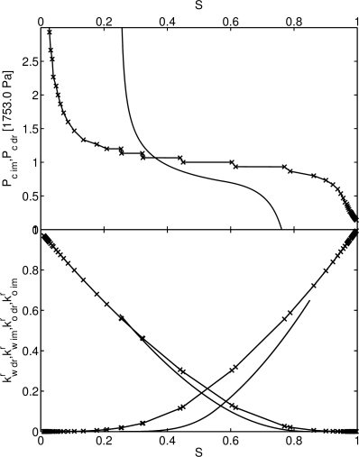
if Leverett-J-function scaling is assumed to to be valid. [7.2.0.3] The rescaled mercury drainage pressure function in the range up to Pa is shown in the upper part of Figure 2 with crosses. [7.2.0.4] For subsequent computations the imbibition curve and the relative permeabilties shown in Figure 2 had to be assumed theoretically, because experimental data were not available. [7.2.0.5] The particular choice for their functional form will influence the numerical results, but is not important for our theoretical argument. [page 8, §0]    [8.1.0.1] The fluid viscosities were

			(48a)
			(48b)

for water denoted and -decane denoted as .

[8.1.1.1] The capillary desaturation experiments in [5] were performed not on the full sample , but on a small subset of . [8.1.1.2] That cylindrical subsample had

			(49a)
			(49b)
			(49c)

where denotes the cross sectional area .
3: Assuming perfect isotropy the dimensionless aspect ratio matrix becomes diagonal with according to eq. (28) in [40]. Because of the ratio of it should be kept in mind that geometric factors can change the force balance by an order of magnitude.

[8.1.2.1] The resulting microscopic capillary numbers were

(50)

with .
4: These capillary numbers differ from those shown in Figure 1 of [5] by a factor .
[8.1.2.2] To compute the macroscopic capillary number from (28) the characteristic pressure is taken from the rescaled drainage curve in the upper part of Figure 2 as

(51)

[8.1.2.3] With this the macroscopic capillary numbers for the -sample are

(52)

for , while

(53)

for the -sample. [8.1.2.4] Note, that the width of the capillary fringe of water

(54)

is around , where is the density of water and is the acceleration of gravity.

[8.1.3.1] Figure 3 compares the experimental observations to the theoretical predictions. [8.1.3.2] Assuming to be fixed, the theoretically predicted capillary desaturation curve for fixed force balance is obtained from the solution of eq. (27)

(55)

as . [8.1.3.3] Figure 3 shows two capillary desaturation curves for water injection into continuous oil according to the CO/WI-protocol (36). [8.1.3.4] One curve (crosses) represents drainage, while the solid curve represents imbibition. [8.2.0.1] Crosses are computed using the rescaled mercury drainage pressures and relative permeabilities for drainage shown in Fig. 2. [8.2.0.2] The solid curve without symbols is computed from the imbibition curves in Fig. 2. [8.2.0.3] The values of and are indicated by dashed horizontal lines.

[8.2.1.1] If all assumptions underlying the traditional equations and the derivations of hold true, then the experimental results are expected to fall in between the two limiting drainage and imbibition curves. [8.2.1.2] To test this expectation Figure 3 shows three experimental capillary desaturation correlations. [8.2.1.3] The experimental values with are plotted as squares against from eq. (50), as triangles against from eq. (53), and as circles against from eq. (52). [8.2.1.4] This comparison between theory and experiment rules out the use of microscopic capillary number as abscissa in capillary desaturation curves. [8.2.1.5] The misleading use of this number is still widely spread in current literature although it has been criticized already in [9, 32]. [8.2.1.6] The comparison with confirms the predictions of traditional two phase flow theory as far as orders of magnitude are concerned. [8.2.1.7] However, it must be emphasized that the comparison uses the CO/WI-protocol for theory, but the DO/IWI/G-protocol for experiment. [8.2.1.8] The theoretical predictions restrict capillary desaturation curves to the region . [8.2.1.9] This prediction is a consequence of the fact that the traditional theory cannot account for disconnected nonpercolating fluid parts. [page 9, §0]    [9.1.0.1] Figure 3 represents, to the best of our knowledge, the first example in which bounds for capillary desaturation curves have been predicted based solely on the constitutive functions of the traditional two phase flow theory.

[9.1.1.1] This subsection introduces for the first time continuous mode capillary saturation experiments in analogy to capillary desaturation experiments. [9.1.1.2] The new saturation protocol is defined as

					(56a)
					(56b)
					(56c)
					(56d)

where . [9.1.1.3] For each fixed the time is chosen such that

(57)

holds, i.e. such that the water production has ceased. [9.1.1.4] The saturation protocol (56) will be referred to as CO/OI-protocol (continuous oil/oil injection). [9.1.1.5] To the best of our knowledge such capillary saturation experiments with CO/OI-protocol have not been performed.

[9.1.2.1] During the CO/OI-protocol the water phase is kept at a sufficiently high ambient pressure so that water can enter the sample while oil is injected. [9.1.2.2] If the ambient pressure is sufficiently high and the oil injection rates are small, the resulting displacement process is expected to show strongly interacting mesoscopic cluster dynamics with numerous breakup and coalescence processes of mesoscopic clusters.

[9.1.3.1] Applying the theoretical prediction from eq. (27) yields capillary saturation curves for fixed force balance from solutions of the equation

(58)

as analogous to capillary desaturation curves shown in Figure 3. [9.1.3.2] The theoretically predicted bounding capillary saturations curves for drainage (crosses) and imbibition (solid curve) are displayed in Figure 4 using again the function shown in Figure 2. [9.1.3.3] Experiments following the CO/OI-protocol are expected to fall in between these two limiting curves. [9.1.3.4] Figure 4 shows that the region between the curves becomes narrow for or for the chosen parameters. [9.1.3.5] In this region strongly interacting mesoscopic clusters are expected to arise from strongly fluctuating breakup ond coalescence of oil ganglia. [9.1.3.6] This expectation is consistent with theoretical network modeling in [44] and with recent experimental observations of two temporal regimes of percolating and nonpercolating fluid flow during imbibition into Gildehauser sandstone in [45].