Appendix C Distributions
[page 65, §1]
[65.1.1] Distributions are generalized functions [31].
[65.1.2] They were invented to overcome
the differentiability requirements for functions in analysis
and mathematical physics [105, 63].
[65.1.3] Distribution theory has also a physical origin.
[65.1.4] A physical observable ![]() can never be measured at a point
can never be measured at a point ![]() because
every measurement apparatus averages over a small volume
around
because
every measurement apparatus averages over a small volume
around ![]() [115].
[65.1.5] This ‘‘smearing out’’ can be modelled as an integration
with smooth ‘‘test functions’’ having compact support.
[115].
[65.1.5] This ‘‘smearing out’’ can be modelled as an integration
with smooth ‘‘test functions’’ having compact support.
[65.2.1] Let ![]() denote the space of admissible test functions.
[65.2.2] Commonly used test function spaces are
denote the space of admissible test functions.
[65.2.2] Commonly used test function spaces are
![]() , the space of infinitely often differentiable
functions,
, the space of infinitely often differentiable
functions,
![]() ,
the space of smooth functions with compact support (see (B.5)),
,
the space of smooth functions with compact support (see (B.5)),
![]() ,
the space of smooth functions vanishing at infinity (see (B.3)),
or the so called Schwartz space
,
the space of smooth functions vanishing at infinity (see (B.3)),
or the so called Schwartz space ![]() of smooth functions
decreasing rapidly at infinity (see (B.21)).
of smooth functions
decreasing rapidly at infinity (see (B.21)).
[65.3.1] A distribution ![]() is a linear and continuous mapping that maps
is a linear and continuous mapping that maps
![]() to a real (
to a real (![]() )
or complex (
)
or complex (![]() ) number
12 (This is a footnote:) 12For vector valued distributions see [106].
[65.3.2] There exists a canonical correspondence
between functions and distributions.
[65.3.3] More precisely, for every locally integrable function
) number
12 (This is a footnote:) 12For vector valued distributions see [106].
[65.3.2] There exists a canonical correspondence
between functions and distributions.
[65.3.3] More precisely, for every locally integrable function
![]() there exists a distribution
there exists a distribution ![]() (often also denoted with the same symbol
(often also denoted with the same symbol ![]() )
defined by
)
defined by
| (C.1) |
for every test function ![]() .
[65.3.4] Distributions that can be written in this way are called
regular distributions.
[65.3.5] Distributions that are not regular are sometimes called singular.
[65.3.6] The mapping
.
[65.3.4] Distributions that can be written in this way are called
regular distributions.
[65.3.5] Distributions that are not regular are sometimes called singular.
[65.3.6] The mapping ![]() that assigns to a locally
integrable
that assigns to a locally
integrable ![]() its associated distribution is injective and
continuous.
[65.3.7] The set of distributions is again a vector space, namely
the dual space of the vector space of test functions, and
it is denoted as
its associated distribution is injective and
continuous.
[65.3.7] The set of distributions is again a vector space, namely
the dual space of the vector space of test functions, and
it is denoted as ![]() where
where ![]() is the test function
space.
is the test function
space.
[page 66, §1]
[66.1.1] Important examples for singular distributions are the
Dirac ![]() -function and its derivatives.
[66.1.2] They are defined by the rules
-function and its derivatives.
[66.1.2] They are defined by the rules
| (C.2) | |||
| (C.3) |
for every test function ![]() and
and ![]() .
[66.1.3] Clearly,
.
[66.1.3] Clearly, ![]() is not a function, because if it were a
function, then
is not a function, because if it were a
function, then ![]() would have to hold.
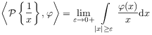
[66.1.4] Another example for a singular distribution is
the finite part or principal value
would have to hold.
[66.1.4] Another example for a singular distribution is
the finite part or principal value ![]() of
of ![]() .
[66.1.5] It is defined by
.
[66.1.5] It is defined by
 |
(C.4) |
for ![]() .
[66.1.6] It is a singular distribution on
.
[66.1.6] It is a singular distribution on ![]() , but regular on
, but regular on
![]() where it coincides
with the function
where it coincides
with the function ![]() .
.
[66.2.1] Equation (C.2) illustrates how distributions circumvent the limitations of differentiation for ordinary functions. [66.2.2] The basic idea is the formula for partial integration
| (C.5) |
valid for ![]() ,
, ![]() ,
,
![]() and
and ![]() an open set.
[66.2.3] The formula is proved by extending
an open set.
[66.2.3] The formula is proved by extending ![]() as
as ![]() to all
of
to all
of ![]() and using Leibniz’ product rule.
[66.2.4] Rewriting the formula as
and using Leibniz’ product rule.
[66.2.4] Rewriting the formula as
| (C.6) |
suggests to view ![]() again as a linear continuous
mapping (integral) on a space
again as a linear continuous
mapping (integral) on a space ![]() of test functions
of test functions
![]() .
[66.2.5] Then the formula is a rule for differentiating
.
[66.2.5] Then the formula is a rule for differentiating ![]() given that
given that ![]() is differentiable.
is differentiable.
[66.3.1] Distributions on the test function space ![]() are called tempered distributions.
[66.3.2] The space of tempered distributions is the dual space
are called tempered distributions.
[66.3.2] The space of tempered distributions is the dual space
![]() .
[66.3.3] Tempered distributions generalize locally integrable
functions growing at most polynomially for
.
[66.3.3] Tempered distributions generalize locally integrable
functions growing at most polynomially for ![]() .
[66.3.4] All distributions with compact support are tempered.
Square integrable functions are tempered distributions.
[66.3.5] The derivative of a tempered distribution is again a
tempered distribution.
[66.3.6]
.
[66.3.4] All distributions with compact support are tempered.
Square integrable functions are tempered distributions.
[66.3.5] The derivative of a tempered distribution is again a
tempered distribution.
[66.3.6] ![]() is dense in
is dense in ![]() for all
for all ![]() but not in
but not in ![]() .
[66.3.7] The Fourier transform and its inverse are continous maps of
the Schwartz space onto itself.
[66.3.8] A distribution
.
[66.3.7] The Fourier transform and its inverse are continous maps of
the Schwartz space onto itself.
[66.3.8] A distribution ![]() belongs to
belongs to ![]() if and
only if it is the derivative of a continuous function with slow
growth, i.e. it is of the form
if and
only if it is the derivative of a continuous function with slow
growth, i.e. it is of the form
![]()
[page 67, §0]
where ![]() ,
, ![]() and
and ![]() is a bounded
continuous function on
is a bounded
continuous function on ![]() .
[67.0.1] Note that the exponential function is not a tempered distribution.
.
[67.0.1] Note that the exponential function is not a tempered distribution.
[67.1.1] A distribution ![]() is said to have
compact support
if there exists a compact subset
is said to have
compact support
if there exists a compact subset ![]() such that
such that
![]() for all test functions
with
for all test functions
with ![]() .
[67.1.2] The Dirac
.
[67.1.2] The Dirac ![]() -function is an example.
[67.1.3]
Other examples are Radon measures on a compact set
-function is an example.
[67.1.3]
Other examples are Radon measures on a compact set ![]() .
[67.1.4] They can be described as linear functionals
on
.
[67.1.4] They can be described as linear functionals
on ![]() .
[67.1.5] If the set
.
[67.1.5] If the set ![]() is sufficiently regular (e.g. if it is the
closure of a region with piecewise smooth boundary)
then every distribution with compact support in
is sufficiently regular (e.g. if it is the
closure of a region with piecewise smooth boundary)
then every distribution with compact support in ![]() can be written in the form
can be written in the form
| (C.7) |
where ![]() ,
, ![]() is a multiindex,
is a multiindex,
![]() and
and ![]() are continuous functions of
compact support.
[67.1.6] Here
are continuous functions of
compact support.
[67.1.6] Here ![]() and the partial derivatives in
and the partial derivatives in ![]() are
distributional derivatives defined above.
[67.1.7] A special case are distributions with support in a single
point taken as
are
distributional derivatives defined above.
[67.1.7] A special case are distributions with support in a single
point taken as ![]() .
[67.1.8] Any such distributions can be written in the form
.
[67.1.8] Any such distributions can be written in the form
| (C.8) |
where ![]() is the Dirac
is the Dirac ![]() -function and
-function and ![]() are constants.
are constants.
[67.2.1] The multiplication of a distribution ![]() with a smooth function
with a smooth function ![]() is defined by the formula
is defined by the formula
![]() where
where ![]() .
[67.2.2] A combination of multiplication by a smooth function
and differentiation allows to define differential
operators
.
[67.2.2] A combination of multiplication by a smooth function
and differentiation allows to define differential
operators
| (C.9) |
with smooth ![]() .
[67.2.3] They are well defined for all distributions in
.
[67.2.3] They are well defined for all distributions in
![]() .
.
[67.3.1] A distribution is called homogeneous of degree ![]() if
if
| (C.10) |
for all ![]() .
[67.3.2] Here
.
[67.3.2] Here ![]() is the standard definition.
[67.3.3] The Dirac
is the standard definition.
[67.3.3] The Dirac ![]() -distribution is homogeneous of degree
-distribution is homogeneous of degree ![]() .
[67.3.4] For regular distributions the definition coincides with
homogeneity of functions
.
[67.3.4] For regular distributions the definition coincides with
homogeneity of functions ![]() .
[67.3.5] The convolution kernels
.
[67.3.5] The convolution kernels ![]() from eq. (2.39)
are homogeneous of degree
from eq. (2.39)
are homogeneous of degree ![]() .
[67.3.6] Homogeneous distributions remain homogeneous under
differentiation.
[67.3.7] A homogeneous locally integrable function
.
[67.3.6] Homogeneous distributions remain homogeneous under
differentiation.
[67.3.7] A homogeneous locally integrable function ![]() on
on ![]() of degree
of degree ![]() can be extended to homogeneous distributions
can be extended to homogeneous distributions ![]() on all
of
on all
of ![]() .
[67.3.8] The degree of homogeneity of
.
[67.3.8] The degree of homogeneity of ![]() must again be
must again be ![]() .
[67.3.9] As long as
.
[67.3.9] As long as ![]() the integral
the integral
| (C.11) |
[page 68, §0]
which converges absolutely for ![]() can be
used to define
can be
used to define ![]() by analytic continuation
from the region
by analytic continuation
from the region ![]() to the point
to the point ![]() .
[68.0.1] For
.
[68.0.1] For ![]() , however, this is not
always possible.
[68.0.2] An example is the function
, however, this is not
always possible.
[68.0.2] An example is the function ![]() on
on ![]() .
[68.0.3] It cannot be extended to a homogeneous distribution of degree
.
[68.0.3] It cannot be extended to a homogeneous distribution of degree ![]() on all of
on all of ![]() .
.
[68.1.1] For ![]() and
and ![]() their tensor product is the function
their tensor product is the function ![]() defined on
defined on ![]() .
[68.1.2] The function
.
[68.1.2] The function ![]() gives a functional
gives a functional
| (C.12) |
for ![]() .
[68.1.3] For two distributions this formula defines the their tensor product.
[68.1.4] An example is a measure
.
[68.1.3] For two distributions this formula defines the their tensor product.
[68.1.4] An example is a measure ![]() concentrated on the
surface
concentrated on the
surface ![]() in
in ![]() where
where ![]() is a measure
on
is a measure
on ![]() .
[68.1.5] The convolution of distribution defined in the main text (see eq.
(2.52) can then be defined by the formula
.
[68.1.5] The convolution of distribution defined in the main text (see eq.
(2.52) can then be defined by the formula
| (C.13) |
whenever one of the distributions ![]() or
or ![]() has compact support.
has compact support.
