2.2 Mathematical Introduction to Fractional Derivatives
[22.1.1] The brief historical introduction has shown that fractional derivatives may be defined in numerous ways. [22.1.2] A natural and frequently used approach starts from repeated integration and extends it to fractional integrals. [22.1.3] Fractional derivatives are then defined either by continuation of fractional integrals to negative order (following Leibniz’ ideas [73]), or by integer order derivatives of fractional integrals (as suggested by Riemann [96]).
2.2.1 Fractional Integrals
2.2.1.1 Iterated Integrals
[22.2.1] Consider a locally integrable1 (This is a footnote:) 1
A function ![]() is called locally integrable if
it is integrable on all compact subsets
is called locally integrable if
it is integrable on all compact subsets ![]() (see eq.(B.9)).
real valued function
(see eq.(B.9)).
real valued function
![]() whose domain of definition
whose domain of definition
![]() is an interval with
is an interval with
![]() .
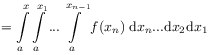
[22.2.2] Integrating
.
[22.2.2] Integrating
[page 23, §0]
![]() times gives the fundamental formula
times gives the fundamental formula
 |
|||
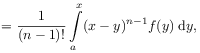 |
(2.27) |
where ![]() and
and ![]() .
[23.0.1] This formula may be proved by induction.
[23.0.2] It reduces
.
[23.0.1] This formula may be proved by induction.
[23.0.2] It reduces ![]() -fold integration to a single
convolution integral (Faltung).
[23.0.3] The subscript
-fold integration to a single
convolution integral (Faltung).
[23.0.3] The subscript ![]() indicates that the integration
has
indicates that the integration
has ![]() as its lower limit.
[23.0.4] An analogous formula holds with
lower limit
as its lower limit.
[23.0.4] An analogous formula holds with
lower limit ![]() and upper limit
and upper limit ![]() .
[23.0.5] In that case the subscript
.
[23.0.5] In that case the subscript ![]() will be used.
will be used.
2.2.1.2 Riemann-Liouville Fractional Integrals
[23.1.1] Equation (2.27) for ![]() -fold
integration can be generalized to
noninteger values of
-fold
integration can be generalized to
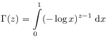
noninteger values of ![]() using the relation
using the relation
![]() where
where
 |
(2.28) |
is Euler’s ![]() -function
defined for all
-function
defined for all ![]() .
.
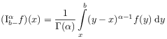
Definition 2.1
[23.2.1] Let ![]() .
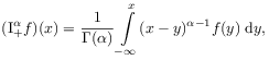
[23.2.2] The Riemann-Liouville fractional integral of order
.
[23.2.2] The Riemann-Liouville fractional integral of order ![]() with lower limit
with lower limit ![]() is defined for locally integrable functions
is defined for locally integrable functions ![]() as
as
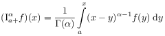 |
(2.29a) | |
| for | ||
 |
(2.29b) | |
for ![]() .
[23.2.4] For
.
[23.2.4] For ![]()
| (2.30) |
completes the definition.
[23.2.5] The definition may be generalized to ![]() with
with ![]() .
.
[page 24, §1]
[24.1.1] Formula (2.29a) appears in
[96, p.363] with ![]() and in
[76, p.8] with
and in
[76, p.8] with ![]() .
[24.1.2] The notation is not standardized.
[24.1.3] Leibniz, Lagrange and Liouville used the
symbol
.
[24.1.2] The notation is not standardized.
[24.1.3] Leibniz, Lagrange and Liouville used the
symbol ![]() [73, 22, 76],
Grünwald wrote
[73, 22, 76],
Grünwald wrote ![]() ,
while Riemann used
,
while Riemann used ![]() [96]
and Most wrote
[96]
and Most wrote ![]() [89].
[24.1.4] The notation in (2.29) is that of [99, 98, 54, 52].
[24.1.5] Modern authors also use
[89].
[24.1.4] The notation in (2.29) is that of [99, 98, 54, 52].
[24.1.5] Modern authors also use ![]() [37],
[37],
![]() [97],
[97],
![]() [94],
[94],
![]() [23],
[23],
![]() [85, 102, 91], or
[85, 102, 91], or
![]() [92]
instead of
[92]
instead of ![]() 2 (This is a footnote:) 2
Some authors [97, 26, 92, 23, 85, 91] employ the
derivative symbol
2 (This is a footnote:) 2
Some authors [97, 26, 92, 23, 85, 91] employ the
derivative symbol ![]() also for integrals, resp.
also for integrals, resp. ![]() for derivatives, to
emphasize the similarity between fractional
integration and differentiation.
If this is done, the choice of Riesz and Feller,
namely
for derivatives, to
emphasize the similarity between fractional
integration and differentiation.
If this is done, the choice of Riesz and Feller,
namely ![]() , seems superior
in the sense that fractional derivatives, similar to integrals, are
nonlocal operators, while integer derivatives are local operators..
, seems superior
in the sense that fractional derivatives, similar to integrals, are
nonlocal operators, while integer derivatives are local operators..
[24.2.1] The fractional integral operators ![]() are commonly
called Riemann-Liouville fractional integrals [99, 98, 94]
although sometimes this name is reserved for
the case
are commonly
called Riemann-Liouville fractional integrals [99, 98, 94]
although sometimes this name is reserved for
the case ![]() [85].
[24.2.2] Their domain of definition is typically chosen
as
[85].
[24.2.2] Their domain of definition is typically chosen
as ![]() or
or
![]() [99, 98, 94].
[24.2.3] For the definition of Lebesgue spaces see the Appendix B.
[24.2.4] If
[99, 98, 94].
[24.2.3] For the definition of Lebesgue spaces see the Appendix B.
[24.2.4] If ![]() then
then ![]() and
and ![]() is finite for almost all
is finite for almost all ![]() .
[24.2.5] If
.
[24.2.5] If ![]() with
with ![]() and
and
![]() then
then ![]() is finite for all
is finite for all ![]() .
[24.2.6] Analogous statements hold for
.
[24.2.6] Analogous statements hold for ![]() [98].
[98].
2.2.1.3 Weyl Fractional Integrals
[24.4.1] Examples (2.5) and (2.6) or
(A.3) and (A.5)
show that Definition 2.1 is well suited for
fractional integration of power series, but not for
functions defined by Fourier series.
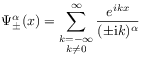
[24.4.2] In fact, if ![]() is a periodic function with period
is a periodic function with period ![]() ,
and3 (This is a footnote:) 3The notation
,
and3 (This is a footnote:) 3The notation ![]() indicates that the sum does not need
to converge, and, if it converges, does not need to
converge to
indicates that the sum does not need
to converge, and, if it converges, does not need to
converge to ![]() .
.
| (2.31) |
then the Riemann-Liouville fractional ![]() will
in general not be periodic.
[24.4.3] For this reason an alternative definition of
fractional integrals was investigated by Weyl [124].
will
in general not be periodic.
[24.4.3] For this reason an alternative definition of
fractional integrals was investigated by Weyl [124].
[24.5.1] Functions on the unit circle ![]() correspond to
correspond to ![]() -periodic functions on the real line.
[24.5.2] Let
-periodic functions on the real line.
[24.5.2] Let ![]() be periodic with period
be periodic with period ![]() and such that
the integral of
and such that
the integral of ![]() over the interval
over the interval ![]() vanishes,
so that
vanishes,
so that ![]() in eq. (2.31).
[24.5.3] Then the integral of
in eq. (2.31).
[24.5.3] Then the integral of ![]() is itself a periodic function,
and the constant of integration can be chosen such that
the integral over
is itself a periodic function,
and the constant of integration can be chosen such that
the integral over ![]() vanishes again.
[24.5.4] Repeating the integration
vanishes again.
[24.5.4] Repeating the integration ![]() times one finds
using (2.6) and the integral representation
times one finds
using (2.6) and the integral representation
[page 25, §0]
![]() of Fourier coefficients
of Fourier coefficients
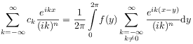 |
(2.32) |
with ![]() .
[25.0.1] Recall the convolution formula [132, p.36]
.
[25.0.1] Recall the convolution formula [132, p.36]
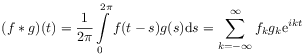 |
(2.33) |
for two periodic functions
![]() and
and
![]() .
[25.0.2] Using eq. (2.33)
and generalizing (2.32)
to noninteger
.
[25.0.2] Using eq. (2.33)
and generalizing (2.32)
to noninteger ![]() suggests the following definition.
[99, 94].
suggests the following definition.
[99, 94].
Definition 2.2
[25.1.1] Let ![]() be periodic
with period
be periodic
with period ![]() and such that its integral over a
period vanishes.
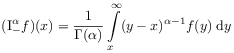
[25.1.2] The Weyl fractional integral of order
and such that its integral over a
period vanishes.
[25.1.2] The Weyl fractional integral of order ![]() is
defined as
is
defined as
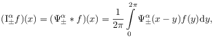 |
(2.34) |
where
 |
(2.35) |
for ![]() .
.
[25.2.1] It can be shown that the series for ![]() converges
and that the Weyl definition coincides with the
Riemann-Liouville definition [133]
converges
and that the Weyl definition coincides with the
Riemann-Liouville definition [133]
 |
(2.36a) | |
| respectively | ||
 |
(2.36b) | |
for ![]() periodic functions whose integral over
a period vanishes.
[25.2.2] This is eq. (2.29) with
periodic functions whose integral over
a period vanishes.
[25.2.2] This is eq. (2.29) with ![]() resp.
resp. ![]() .
[25.2.3] For this reason the Riemann-Liouville
.
[25.2.3] For this reason the Riemann-Liouville
[page 26, §0]
fractional
integrals with limits ![]() ,
,
![]() and
and
![]() ,
are often called Weyl fractional integrals
[24, 99, 85, 94].
,
are often called Weyl fractional integrals
[24, 99, 85, 94].
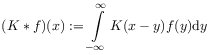
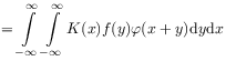
[26.1.1] The Weyl fractional integral may be rewritten as a convolution
| (2.37) |
where the convolution product for
functions on ![]() is defined as4 (This is a footnote:) 4
If
is defined as4 (This is a footnote:) 4
If ![]() then
then ![]() exists for almost all
exists for almost all ![]() and
and ![]() .
[26.1.2] If
.
[26.1.2] If ![]() ,
, ![]() with
with
![]() and
and ![]() then
then
![]() , the space of continuous functions
vanishing at infinity.
, the space of continuous functions
vanishing at infinity.
 |
(2.38) |
and the convolution kernels are defined as
| (2.39) |
for ![]() .
[26.1.3] Here
.
[26.1.3] Here
| (2.40) |
is the Heaviside unit step function,
and ![]() with the convention that
with the convention that
![]() is real for
is real for ![]() .
[26.1.4] For
.
[26.1.4] For ![]() the kernel
the kernel
| (2.41) |
is the Dirac ![]() -function defined in (C.2)
in Appendix C.
[26.1.5] Note that
-function defined in (C.2)
in Appendix C.
[26.1.5] Note that ![]() for
for ![]() .
.
2.2.1.4 Riesz Fractional Integrals
[26.2.1] Riemann-Liouville and Weyl fractional integrals have upper or lower limits of integration, and are sometimes called left-sided resp. right-sided integrals. [26.2.2] A more symmetric definition was advanced in [97].
Definition 2.3
[26.3.1] Let ![]() be locally integrable.
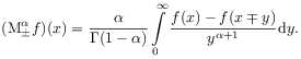
[26.3.2] The Riesz fractional integral or Riesz potential
of order
be locally integrable.
[26.3.2] The Riesz fractional integral or Riesz potential
of order ![]() is defined as the linear combination [99]
is defined as the linear combination [99]
 |
(2.42) |
[27.1.1] Riesz fractional integration may be written as a convolution
| (2.45a) | |||
| (2.45b) |
with the (one-dimensional) Riesz kernels
| (2.46) |
for ![]() , and
, and
| (2.47) |
for ![]() .
[27.1.2] Subsequently, Feller introduced the
generalized Riesz-Feller kernels [26]
.
[27.1.2] Subsequently, Feller introduced the
generalized Riesz-Feller kernels [26]
| (2.48) |
with parameter ![]() .
[27.1.3] The corresponding generalized
Riesz-Feller fractional integral of order
.
[27.1.3] The corresponding generalized
Riesz-Feller fractional integral of order ![]() and type
and type ![]() is defined as
is defined as
| (2.49) |
[27.1.4] This formula interpolates continuously from the Weyl integral
![]() for
for ![]() through the Riesz integral
through the Riesz integral
![]() for
for ![]() to the Weyl integral
to the Weyl integral
![]() for
for ![]() .
[27.1.5] Due to their symmetry Riesz-Feller fractional
integrals are readily generalized to higher dimensions.
.
[27.1.5] Due to their symmetry Riesz-Feller fractional
integrals are readily generalized to higher dimensions.
[page 28, §1]
2.2.1.5 Fractional Integrals of Distributions
[28.1.1] Fractional integration can be extended to distributions
using the convolution formula (2.37) above.
[28.1.2] Distributions are generalized functions [105, 31].
[28.1.3] They are defined as linear functionals on a space ![]() of
conveniently chosen ‘‘test functions’’.
[28.1.4] For every locally integrable function
of
conveniently chosen ‘‘test functions’’.
[28.1.4] For every locally integrable function
![]() there exists a distribution
there exists a distribution ![]() defined by
defined by
 |
(2.50) |
where ![]() is test function from a suitable space
is test function from a suitable space
![]() of test functions.
[28.1.5] By abuse of notation one often writes
of test functions.
[28.1.5] By abuse of notation one often writes
![]() for the associated distribution
for the associated distribution ![]() .
[28.1.6] Distributions that correspond to functions via (2.50)
are called regular distributions.
[28.1.7] Examples for regular distributions are
the convolution kernels
.
[28.1.6] Distributions that correspond to functions via (2.50)
are called regular distributions.
[28.1.7] Examples for regular distributions are
the convolution kernels ![]() defined in (2.39).
[28.1.8] They are locally integrable functions on
defined in (2.39).
[28.1.8] They are locally integrable functions on ![]() when
when ![]() .
[28.1.9] Distributions that are not regular are sometimes called singular.
[28.1.10] An important example for a singular distribution is the
Dirac
.
[28.1.9] Distributions that are not regular are sometimes called singular.
[28.1.10] An important example for a singular distribution is the
Dirac ![]() -function.
[28.1.11] It is defined as
-function.
[28.1.11] It is defined as ![]()
| (2.51) |
for every test function ![]() .
[28.1.12] The test function space
.
[28.1.12] The test function space ![]() is usually chosen as a
subspace of
is usually chosen as a
subspace of ![]() , the space of
infinitely differentiable functions.
[28.1.13] A brief introduction to distributions is given in
Appendix C.
, the space of
infinitely differentiable functions.
[28.1.13] A brief introduction to distributions is given in
Appendix C.
[28.2.1] In order to generalize (2.37) to distributions
one must define the convolution of two distributions.
[28.2.2] To do so one multiplies eq. (2.38) on both sides
with a smooth test function ![]() of
compact support.
[28.2.3] Integrating gives
of
compact support.
[28.2.3] Integrating gives
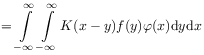 |
|||
 |
|||
| (2.52) |
where the notation ![]() means that the functional
means that the functional ![]() is applied to the function
is applied to the function
![]() for fixed
for fixed ![]() .
[28.2.4] Explicitly, for fixed
.
[28.2.4] Explicitly, for fixed ![]()
 |
(2.53) |
[page 29, §0]
where ![]() .
[29.0.1] Equation (2.52) can be used as a definition
for the convolution of distributions provided that the
right hand side has meaning.
[29.0.2] This is not always the case as the
counterexample
.
[29.0.1] Equation (2.52) can be used as a definition
for the convolution of distributions provided that the
right hand side has meaning.
[29.0.2] This is not always the case as the
counterexample ![]() shows.
[29.0.3] In general the convolution product is not associative
(see eq. (2.113)).
[29.0.4] However, associative and commutative convolution
algebras exist [21].
[29.0.5] Equation (2.52) is always meaningful
when
shows.
[29.0.3] In general the convolution product is not associative
(see eq. (2.113)).
[29.0.4] However, associative and commutative convolution
algebras exist [21].
[29.0.5] Equation (2.52) is always meaningful
when ![]() or
or ![]() is compact [63].
[29.0.6] Another case
is when
is compact [63].
[29.0.6] Another case
is when ![]() and
and ![]() have support in
have support in ![]() .
[29.0.7] This will be assumed in the following.
.
[29.0.7] This will be assumed in the following.
Definition 2.4
[29.1.1] Let ![]() be a distribution
be a distribution ![]() with
with ![]() .
[29.1.2] Then its fractional integral is the distribution
.
[29.1.2] Then its fractional integral is the distribution
![]() defined as
defined as
| (2.54) |
for ![]() .
[29.1.3] It has support in
.
[29.1.3] It has support in ![]() .
.
[29.2.1] If ![]() with
with ![]() then also
then also ![]() with
with ![]() .
.
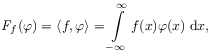
2.2.1.6 Integral Transforms
[29.3.1] The Fourier transformation is defined as
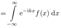 |
(2.55) |
for functions ![]() .
[29.3.2] Then
.
[29.3.2] Then
| (2.56) |
holds for ![]() by virtue of the convolution theorem.
[29.3.3] The equation cannot be extended directly to
by virtue of the convolution theorem.
[29.3.3] The equation cannot be extended directly to ![]() because the Fourier integral on the left hand side may not
exist.
[29.3.4] Consider e.g.
because the Fourier integral on the left hand side may not
exist.
[29.3.4] Consider e.g. ![]() and
and ![]() .
[29.3.5] Then
.
[29.3.5] Then ![]() const as
const as ![]() and
and
![]() does not exist [94].
[29.3.6] Equation (2.56) can be extended to all
does not exist [94].
[29.3.6] Equation (2.56) can be extended to all ![]() with
with
![]() for functions in the so called Lizorkin space
[99, p.148] defined as the space of functions
for functions in the so called Lizorkin space
[99, p.148] defined as the space of functions ![]() such that
such that ![]() for all
for all ![]() .
.
[29.4.1] For the Riesz potentials one has
| (2.57a) | |||
| (2.57b) |
for functions in Lizorkin space.
[page 30, §1] [30.1.1] The Laplace transform is defined as
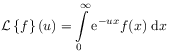 |
(2.58) |
for locally integrable functions ![]() .
[30.1.2] Now
.
[30.1.2] Now
| (2.59) |
by the convolution theorem for Laplace transforms.
[30.1.3] The Laplace transform of ![]() leads to a more complicated operator.
leads to a more complicated operator.
2.2.1.7 Fractional Integration by Parts
[30.2.1] If ![]() with
with ![]() ,
, ![]() and
and
![]() ,
, ![]() for
for ![]() then
the formula
then
the formula
 |
(2.60) |
holds.
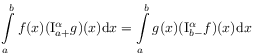
[30.2.2] The formula is known as fractional integration by parts [99].
[30.2.3] For ![]() with
with ![]() and
and ![]() the analogous formula
the analogous formula
 |
(2.61) |
holds for Weyl fractional integrals.
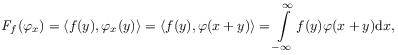
[30.3.1] These formulae provide a second method of generalizing fractional integration to distributions. [30.3.2] Equation (2.60) may be read as
| (2.62) |
for a distribution ![]() and a test function
and a test function ![]() .
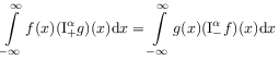
[30.3.3] It shows that right- and left-sided fractional integrals
are adjoint operators.
[30.3.4] The formula may be viewed as a definition
of the fractional integral
.
[30.3.3] It shows that right- and left-sided fractional integrals
are adjoint operators.
[30.3.4] The formula may be viewed as a definition
of the fractional integral ![]() of a distribution
provided that the operator
of a distribution
provided that the operator ![]() maps the test function
space into itself.
maps the test function
space into itself.
2.2.1.8 Hardy-Littlewood Theorem
[30.4.1] The mapping properties of convolutions can be studied
with the help of Youngs inequality.
Let ![]() obey
obey ![]() and
and
![]() .
[30.4.2] If
.
[30.4.2] If ![]() and
and ![]() then
then
![]() and Youngs inequality
and Youngs inequality
![]() holds.
[30.4.3] It follows that
holds.
[30.4.3] It follows that
![]() if
if
[page 31, §0]
![]() and
and ![]() with
with
![]() .
[31.0.1] The Hardy-Littlewood theorem states that these estimates
remain valid for
.
[31.0.1] The Hardy-Littlewood theorem states that these estimates
remain valid for ![]() although these kernels
do not belong to any
although these kernels
do not belong to any ![]() -space
[37, 38].
[31.0.2] The theorem was generalized to higher dimensions
by Sobolev in 1938, and is also known as the Hardy-Littlewood-Sobolev
inequality (see [37, 38, 113, 63]).
-space
[37, 38].
[31.0.2] The theorem was generalized to higher dimensions
by Sobolev in 1938, and is also known as the Hardy-Littlewood-Sobolev
inequality (see [37, 38, 113, 63]).
Theorem 2.5
[31.1.1] Let ![]() ,
, ![]() ,
, ![]() .
[31.1.2] Then
.
[31.1.2] Then ![]() are bounded linear operators
from
are bounded linear operators
from ![]() to
to ![]() with
with ![]() ,i.e.
there exists a constant
,i.e.
there exists a constant ![]() independent of
independent of ![]() such that
such that
![]() .
.
2.2.1.9 Additivity
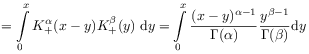
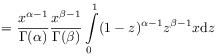
[31.2.1] The basic composition law for fractional integrals follows from
 |
|||
 |
|||
| (2.63) |
where Euler’s Beta-function
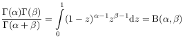 |
(2.64) |
was used. [31.2.2] This implies the semigroup law for exponents
| (2.65) |
also called additivity law. [31.2.3] It holds for Riemann-Liouville, Weyl and Riesz-Feller fractional integrals of functions.
2.2.2 Fractional Derivatives
2.2.2.1 Riemann-Liouville Fractional Derivatives
[31.3.1] Riemann [96, p.341] suggested to define fractional derivatives as integer order derivatives of fractional integrals.
Definition 2.6
[31.4.1] Let ![]() .
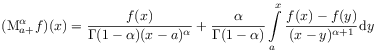
[31.4.2] The Riemann-Liouville fractional derivative of order
.
[31.4.2] The Riemann-Liouville fractional derivative of order ![]() with lower limit
with lower limit ![]() (resp. upper limit
(resp. upper limit ![]() )
is defined for
)
is defined for
[page 32, §0]
functions such that ![]() and
and
![]() as
as
| (2.66) |
and ![]() for
for ![]() .
[32.0.1] For
.
[32.0.1] For ![]() the definition is extended
for functions
the definition is extended
for functions ![]() with
with
![]() as
as
| (2.67) |
where5 (This is a footnote:) 5![]() is the largest integer smaller than
is the largest integer smaller than ![]() .
.
![]() is smallest integer larger than
is smallest integer larger than ![]() .
.
[32.1.1] Here ![]() denotes a Sobolev space defined in (B.17).
[32.1.2] For
denotes a Sobolev space defined in (B.17).
[32.1.2] For ![]() the space
the space ![]() coincides
with the space of absolutely continuous functions.
coincides
with the space of absolutely continuous functions.
[32.2.1] The notation for fractional derivatives is not
standardized6 (This is a footnote:) 6see footnote 2.1.
[32.2.2] Leibniz and Euler used ![]() [73, 72, 25]
Riemann wrote
[73, 72, 25]
Riemann wrote ![]() [96],
Liouville preferred
[96],
Liouville preferred ![]() [76],
Grünwald used
[76],
Grünwald used ![]() or
or
![]() [34],
Marchaud wrote
[34],
Marchaud wrote ![]() , and
Hardy-Littlewood used an index
, and
Hardy-Littlewood used an index ![]() [37].
[32.2.3] The notation in (2.67) follows [99, 98, 54, 52].
Modern authors also use
[37].
[32.2.3] The notation in (2.67) follows [99, 98, 54, 52].
Modern authors also use
![]() [97],
[97],
![]() [23],
[23],
![]() [94, 85, 102],
[94, 85, 102],
![]() [129, 102],
[129, 102],
![]() [92]
instead of
[92]
instead of ![]() .
.
[32.3.1] Let ![]() be absolutely continuous on the finite interval
be absolutely continuous on the finite interval ![]() .
[32.3.2] Then, its derivative
.
[32.3.2] Then, its derivative ![]() exists almost everywhere on
exists almost everywhere on
![]() with
with ![]() , and
the function
, and
the function ![]() can be
written as
can be
written as
 |
(2.68) |
Substituting this into ![]() gives
gives
| (2.69) |
where commutativity of ![]() and
and ![]() was used.
[32.3.3] It follows that
was used.
[32.3.3] It follows that
| (2.70) |
for ![]() .
[32.3.4] Above, the notations
.
[32.3.4] Above, the notations
| (2.71) |
were used for the first order derivative.
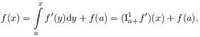
[page 33, §1] [33.1.1] This observation suggests to introduce a modified Riemann-Liouville fractional derivative through
 |
(2.72) |
where ![]() .
[33.1.2] Note, that
.
[33.1.2] Note, that ![]() must be at least
must be at least ![]() -times differentiable.
[33.1.3] Formula (2.72) is due to Liouville [76, p.10]
(see eq. (2.18) above),
but nowadays sometimes named after Caputo [17].
-times differentiable.
[33.1.3] Formula (2.72) is due to Liouville [76, p.10]
(see eq. (2.18) above),
but nowadays sometimes named after Caputo [17].
Theorem 2.7
[33.2.2] For ![]() with
with ![]() the Riemann-Liouville fractional derivative
the Riemann-Liouville fractional derivative
![]() exists almost everywhere
for
exists almost everywhere
for ![]() .
[33.2.3] It can be written as
.
[33.2.3] It can be written as
| (2.73) |
in terms of the Liouville(-Caputo) derivative defined in (2.72).
[33.3.1] The Riemann-Liouville fractional derivative is the left inverse of Riemann-Liouville fractional integrals. [33.3.2] More specifically, [99, p.44]
Theorem 2.8
[33.3.3] Let ![]() .
[33.3.4] Then
.
[33.3.4] Then
| (2.74) |
holds for all ![]() with
with ![]() .
.
[33.4.1] For the right inverses of fractional integrals one finds
Theorem 2.9
[33.4.2] Let ![]() and
and ![]() .
[33.4.3] If in addition
.
[33.4.3] If in addition ![]() where
where
![]() then
then
| (2.75) |
holds.
[33.4.4] For ![]() this becomes
this becomes
| (2.76) |
[33.5.1] The last theorem implies that for ![]() and
and ![]() with
with
![]() the equality
the equality
| (2.77) |
[page 34, §0] holds only if
| (2.78a) | ||
| and | ||
| (2.78b) | ||
for all ![]() .
[34.0.1] Note that the existence of
.
[34.0.1] Note that the existence of ![]() in
eq. (2.77) does not imply that
in
eq. (2.77) does not imply that ![]() can be
written as
can be
written as ![]() for some integrable function
for some integrable function ![]() [99].
[34.0.2] This holds only if both conditions (2.78) are satisfied.
[34.0.3] As an example where one of them fails, consider
the function
[99].
[34.0.2] This holds only if both conditions (2.78) are satisfied.
[34.0.3] As an example where one of them fails, consider
the function ![]() for
for ![]() .
[34.0.4] Then
.
[34.0.4] Then ![]() exists.
[34.0.5] Now
exists.
[34.0.5] Now ![]() so that
(2.78b) fails.
[34.0.6] There does not
exist an integrable
so that
(2.78b) fails.
[34.0.6] There does not
exist an integrable ![]() such that
such that ![]() .
[34.0.7] In fact,
.
[34.0.7] In fact, ![]() corresponds to the
corresponds to the ![]() -distribution
-distribution ![]() .
.
2.2.2.2 General Types of Fractional Derivatives
[34.1.1] Riemann-Liouville fractional derivatives have been generalized in [52, p.433] to fractional derivatives of different types.
Definition 2.10
[34.2.1] The generalized Riemann-Liouville fractional derivative of order
![]() and type
and type ![]() with lower (resp. upper) limit
with lower (resp. upper) limit ![]() is defined as
is defined as
| (2.79) |
for functions such that the expression on the right hand side exists.
[34.3.1] The type ![]() of a fractional derivative allows to
interpolate continuously from
of a fractional derivative allows to
interpolate continuously from ![]() to
to ![]() .
[34.3.2] A relation between fractional derivatives of the same order
but different types was given in [52, p.434].
.
[34.3.2] A relation between fractional derivatives of the same order
but different types was given in [52, p.434].
2.2.2.3 Marchaud-Hadamard Fractional Derivatives
[34.4.1] Marchaud’s approach [78] is based on Hadamards finite parts of divergent integrals [36]. [34.4.2] The strategy is to define fractional derivatives as analytic continuation of fractional integrals to negative orders. [see [99, p.225]]
Definition 2.11
[34.5.1] Let ![]() and
and ![]() .
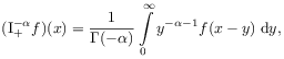
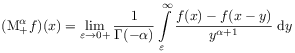
[34.5.2] The
Marchaud fractional derivative of order
.
[34.5.2] The
Marchaud fractional derivative of order ![]() with lower limit
with lower limit ![]() is defined as
is defined as
 |
(2.80) |
[page 35, §0]
and the
Marchaud fractional derivative of order ![]() with upper limit
with upper limit ![]() is defined as
is defined as
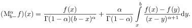 |
(2.81) |
[35.0.1] For ![]() (resp.
(resp. ![]() ) the definition is
) the definition is
 |
(2.82) |
[35.0.2] The definition is completed with ![]() for all
variants.
for all
variants.
[35.1.1] The idea of Marchaud’s method is to extend
the Riemann-Liouville integral from ![]() to
to ![]() ,
and to define
,
and to define
 |
(2.83) |
where ![]() .
[35.1.2] However, this is not possible because the
integral in (2.83) diverges.
[35.1.3] The idea is to subtract the divergent part of the integral,
.
[35.1.2] However, this is not possible because the
integral in (2.83) diverges.
[35.1.3] The idea is to subtract the divergent part of the integral,
| (2.84) |
obtained by setting ![]() for
for ![]() .
[35.1.4] Subtracting (2.83) from (2.84) for
.
[35.1.4] Subtracting (2.83) from (2.84) for
![]() suggests the definition
suggests the definition
 |
(2.85) |
[35.1.5] Formal integration by parts leads to ![]() ,
showing that this definition contains the Riemann-Liouville
definition.
,
showing that this definition contains the Riemann-Liouville
definition.
[35.2.1] The definition may be extended to ![]() in two ways.
[35.2.2] The first consists in applying (2.85) to the
in two ways.
[35.2.2] The first consists in applying (2.85) to the ![]() -th
derivative
-th
derivative ![]() for
for ![]() .
[35.2.3] The second possibility is to regard
.
[35.2.3] The second possibility is to regard ![]() as
a first order difference, and to generalize to
as
a first order difference, and to generalize to ![]() -th order
differences.
[35.2.4] The
-th order
differences.
[35.2.4] The ![]() -th order difference is
-th order difference is
| (2.86) |
where ![]() is the identity operator and
is the identity operator and
| (2.87) |
[page 36, §0]
is the translation operator.
[36.0.1] The Marchaud fractional derivative can then be
extended to ![]() through [94, 98]
through [94, 98]
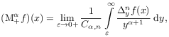 |
(2.88) |
where
 |
(2.89) |
where the limit may be taken in the sense of pointwise or norm convergence.
[36.1.1] The Marchaud derivatives ![]() are defined for a wider class of functions than
Weyl derivatives
are defined for a wider class of functions than
Weyl derivatives ![]() .
[36.1.2] As an example consider the function
.
[36.1.2] As an example consider the function ![]() const.
const.
[36.2.1] Let ![]() be such that there exists a function
be such that there exists a function
![]() with
with ![]() .
[36.2.2] Then
the Riemann-Liouville derivative and
the Marchaud derivative coincide almost everywhere, i.e.
.
[36.2.2] Then
the Riemann-Liouville derivative and
the Marchaud derivative coincide almost everywhere, i.e.
![]() for almost
all
for almost
all ![]() [99, p.228].
[99, p.228].
2.2.2.4 Weyl Fractional Derivatives
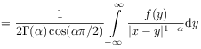
[36.3.1] There are two kinds of Weyl fractional derivatives for periodic functions. [36.3.2] The Weyl-Liouville fractional derivative is defined as [99, p.351],[94]
| (2.90) |
for ![]() where the Weyl integral
where the Weyl integral ![]() was defined
in (2.34).
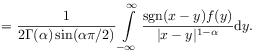
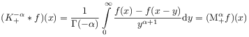
[36.3.3] The Weyl-Marchaud fractional derivative is defined
as [99, p.352],[94]
was defined
in (2.34).
[36.3.3] The Weyl-Marchaud fractional derivative is defined
as [99, p.352],[94]
(y)\mathrm{d}y](mi/mi121.png) |
(2.91) |
for ![]() where
where ![]() is defined in eq. (2.35).
[36.3.4] The Weyl derivatives are defined for periodic functions of with zero mean
in
is defined in eq. (2.35).
[36.3.4] The Weyl derivatives are defined for periodic functions of with zero mean
in ![]() where
where ![]() .
[36.3.5] In this space
.
[36.3.5] In this space ![]() ,
i.e. the Weyl-Liouville and Weyl-Marchaud form coincide [99].
[36.3.6] As for fractional integrals, it can be shown that the
Weyl-Liouville derivative
,
i.e. the Weyl-Liouville and Weyl-Marchaud form coincide [99].
[36.3.6] As for fractional integrals, it can be shown that the
Weyl-Liouville derivative ![]()
 |
(2.92) |
coincides with the Riemann-Liouville derivative with
lower limit ![]() .
[36.3.7] In addition one has the equivalence
.
[36.3.7] In addition one has the equivalence ![]() with the Marchaud-Hadamard fractional derivative in a suitable
sense [99, p.357].
with the Marchaud-Hadamard fractional derivative in a suitable
sense [99, p.357].
[page 37, §1]
2.2.2.5 Riesz Fractional Derivatives
[37.1.1] To define the Riesz fractional derivative as integer derivatives of Riesz potentials consider the Fourier transforms
| (2.93) |
| (2.94) |
for ![]() .
[37.1.2] Comparing this to eq. (2.57)
suggests to consider
.
[37.1.2] Comparing this to eq. (2.57)
suggests to consider
| (2.95) |
as a candidate for the Riesz fractional derivative.
[37.2.1] Following [94] the
strong Riesz fractional derivative of order ![]()
![]() of a function
of a function ![]() ,
, ![]() ,
is defined through the limit
,
is defined through the limit
| (2.96) |
whenever it exists. [37.2.2] The convolution kernel defined as
| (2.97) |
is obtained from eq. (2.95).
[37.2.3] Indeed, this definition is equivalent to eq. (2.94).
[37.2.4] A function ![]() where
where ![]() has a strong Riesz derivative of order
has a strong Riesz derivative of order ![]() if and only
if there exsists a function
if and only
if there exsists a function ![]() such that
such that
![]() .
[37.2.5] Then
.
[37.2.5] Then ![]() .
.
2.2.2.6 Grünwald-Letnikov Fractional Derivatives
[37.3.1] The basic idea of the Grünwald approach is to generalize finite difference quotients to noninteger order, and then take the limit to obtain a differential quotient. [37.3.2] The first order derivative is the limit
| (2.98) |
of a difference quotient.
[37.3.3] In the last equality ![]() is the identity operator,
and
is the identity operator,
and
| (2.99) |
is the translation operator.
[37.3.4] Repeated application of ![]() gives
gives
| (2.100) |
[page 38, §0]
where ![]() .
[38.0.1] The second order derivative can then be written as
.
[38.0.1] The second order derivative can then be written as
| (2.101) |
and the ![]() -th derivative
-th derivative
| (2.102) |
which exhibits the similarity with the binomial formula.
[38.0.2] The generalization to noninteger ![]() gives rise to
fractional difference quotients defined through
gives rise to
fractional difference quotients defined through
| (2.103) |
for ![]() .
[38.0.3] These are generally divergent for
.
[38.0.3] These are generally divergent for ![]() .
[38.0.4] For example, if
.
[38.0.4] For example, if ![]() , then
, then
| (2.104) |
diverges as ![]() if
if ![]() .
[38.0.5] Fractional difference quotients were studied in [68].
Note that fractional differences obey [99]
.
[38.0.5] Fractional difference quotients were studied in [68].
Note that fractional differences obey [99]
| (2.105) |
Definition 2.12
[38.1.1] The Grünwald-Letnikov fractional derivative of order ![]() is defined as the limit
is defined as the limit
| (2.106) |
of fractional difference quotients whenever the limit exists. [38.1.2] The Grünwald Letnikov fractional derivative is called pointwise or strong depending on whether the limit is taken pointwise or in the norm of a suitable Banach space.
[38.2.1] For a definition of Banach spaces and their norms see e.g. [128].
[38.3.1] The Grünwald-Letnikov fractional derivative
has been studied for periodic functions in ![]() with
with ![]() in [99, 94].
[38.3.2] It has the following properties.
in [99, 94].
[38.3.2] It has the following properties.
[page 39, §1]
Theorem 2.13
[39.1.1] Let ![]() ,
, ![]() and
and ![]() .
[39.1.2] Then the following statements are equivalent:
.
[39.1.2] Then the following statements are equivalent:
[39.1.3] There exists a function
 such that
 where
where  .
.[39.1.4] There exists a function
such that holds for almost all
  .
.
Theorem 2.14
[39.2.1] Let ![]() ,
, ![]() and
and ![]() .
[39.2.2] Then:
.
[39.2.2] Then:
- implies
 for every
  .
. 
2.2.2.7 Fractional Derivatives of Distributions
[39.3.1] The basic idea for defining fractional differentiation of
distributions is to extend the definition of fractional
integration (2.54) to negative ![]() .
[39.3.2] However, for
.
[39.3.2] However, for ![]() the distribution
the distribution
![]() becomes singular because
becomes singular because ![]() is
not locally integrable in this case.
[39.3.3] The extension of
is
not locally integrable in this case.
[39.3.3] The extension of ![]() to
to ![]() requires
regularization [31, 128, 63].
[39.3.4] It turns out that the regularization exists and is
essentially unique as long as
requires
regularization [31, 128, 63].
[39.3.4] It turns out that the regularization exists and is
essentially unique as long as ![]() .
.
Definition 2.15
[39.4.1] Let ![]() be a distribution
be a distribution ![]() with
with ![]() .
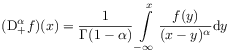
[39.4.2] Then the fractional derivative of order
.
[39.4.2] Then the fractional derivative of order ![]() with lower limit
with lower limit ![]() is the distribution
is the distribution ![]() defined as
defined as
| (2.107) |
where ![]() and
and
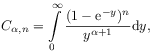
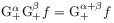
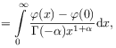
![K_{+}^{\alpha}(x)=\begin{cases}\Theta(x)\displaystyle\frac{x^{{\alpha-1}}}{\Gamma(\alpha)}&,\mathrm{Re}\,\alpha>0\\
&\\
\displaystyle\frac{\mathrm{d}^{N}}{\mathrm{d}x^{N}}\left[\Theta(x)\displaystyle\frac{x^{{\alpha+N-1}}}{\Gamma(\alpha+N)}\right]&,\mathrm{Re}\,\alpha+N>0,N\in\mathbb{N}\end{cases}](mi/mi130.png) |
(2.108) |
is the kernel distribution.
[39.4.3] For ![]() one finds
one finds ![]() and
and ![]() as the identity operator.
[39.4.4] For the
as the identity operator.
[39.4.4] For the ![]() one finds
one finds
| (2.109) |
where ![]() is the
is the ![]() -th derivative
of the
-th derivative
of the ![]() distribution.
distribution.
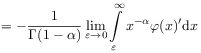
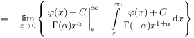
[page 40, §1] [40.1.1] The kernel distribution in (2.108) is
| (2.110) |
for ![]() .
[40.1.2] Its regularized action is
.
[40.1.2] Its regularized action is
| (2.111a) | |||
 |
(2.111b) | ||
 |
(2.111c) | ||
 |
(2.111d) |
where ![]() was assumed in the last step
and the arbitrary constant was chosen as
was assumed in the last step
and the arbitrary constant was chosen as ![]() .
[40.1.3] This choice regularizes the divergent first term in (2.111c).
[40.1.4] If this rule is used for the distributional convolution
.
[40.1.3] This choice regularizes the divergent first term in (2.111c).
[40.1.4] If this rule is used for the distributional convolution
 |
(2.112) |
then the Marchaud-Hadamard form is recovered with ![]() .
.
[40.2.1] It is now possible to show that the convolution of distributions is in general not associative. [40.2.2] A counterexample is
| (2.113) |
where ![]() is the Heaviside step function.
is the Heaviside step function.
[40.3.1] ![]() has support in
has support in ![]() .
[40.3.2] The distributions in
.
[40.3.2] The distributions in ![]() with
with ![]() form a convolution algebra [21] and
one finds [31, 99]
form a convolution algebra [21] and
one finds [31, 99]
Theorem 2.16
[40.3.3] If ![]() with
with ![]() then also
then also ![]() with
with ![]() .
[40.3.4] Moreover, for all
.
[40.3.4] Moreover, for all ![]()
| (2.114) |
with ![]() for
for ![]() .
[40.3.5] For each
.
[40.3.5] For each ![]() with
with ![]() there exists a unique distribution
there exists a unique distribution ![]() with
with ![]() such that
such that
![]() .
.
[page 41, §1] [41.1.1] Note that
| (2.115) |
for all ![]() .
[41.2.1] Also, the differentiation rule
.
[41.2.1] Also, the differentiation rule
| (2.116) |
holds for all ![]() .
[41.2.2] It contains
.
[41.2.2] It contains
| (2.117) |
for all ![]() as a special case.
as a special case.
2.2.2.8 Fractional Derivatives at Their Lower Limit
[41.3.1] All fractional derivatives defined above are nonlocal operators. [41.3.2] A local fractional derivative operator was introduced in [40, 41, 52].
Definition 2.17
[41.4.1] For ![]() the
Riemann-Liouville fractional derivative of order
the
Riemann-Liouville fractional derivative of order ![]() at the lower limit
at the lower limit ![]() is defined by
is defined by
| (2.118) |
whenever the two limits exist and are equal.
[41.4.2] If ![]() exists the function
exists the function ![]() is called
fractionally differentiable at the limit
is called
fractionally differentiable at the limit ![]() .
.
[41.5.1] These operators are useful for the analysis of singularities. [41.5.2] They were applied in [40, 41, 42, 44, 52] to the analysis of singularities in the theory of critical phenomena and to the generalization of Ehrenfests classification of phase transitions. [41.5.3] There is a close relationship to the theory of regularly varying functions [107] as evidenced by the following result [52].
Theorem 2.18
[41.6.1] Let the function ![]() be monotonously increasing with
be monotonously increasing with
![]() and
and ![]() , and such that
, and such that
![]() with
with ![]() and
and ![]() is
also monotonously increasing on a neighbourhood
is
also monotonously increasing on a neighbourhood ![]() for
small
for
small ![]() .
[41.6.2] Let
.
[41.6.2] Let ![]() , let
, let ![]() be a constant and
be a constant and
![]() a slowly varying function for
a slowly varying function for ![]() .
[41.6.3] Then
.
[41.6.3] Then
| (2.119) |
holds if and only if
| (2.120) |
holds.
[page 42, §1]
[42.1.1] A function ![]() is called slowly varying at infinity if
is called slowly varying at infinity if
![]() for all
for all ![]() .
[42.1.2] A function
.
[42.1.2] A function ![]() is called slowly varying at
is called slowly varying at ![]() if
if
![]() is slowly varying at infinity.
is slowly varying at infinity.
2.2.2.9 Fractional Powers of Operators
[42.2.1] The spectral decomposition of selfadjoint operators
is a familiar mathematical tool from quantum mechanics [116].
[42.2.2] Let ![]() denote a selfadjoint operator with domain
denote a selfadjoint operator with domain ![]() and spectral family
and spectral family ![]() on a Hilbert
space
on a Hilbert
space ![]() with scalar product
with scalar product ![]() .
[42.2.3] Then
.
[42.2.3] Then
| (2.121) |
holds for all ![]() .
[42.2.4] Here
.
[42.2.4] Here ![]() is the spectrum of
is the spectrum of ![]() .
[42.2.5] It is then straightforward to define
the fractional power
.
[42.2.5] It is then straightforward to define
the fractional power ![]() by
by
| (2.122) |
on the domain
| (2.123) |
[42.2.6] Similarly, for any measurable
function ![]() the operator
the operator ![]() is
defined with an integrand
is
defined with an integrand ![]() in eq. (2.122).
[42.2.7] This yields an operator calculus that allows to
perform calculations with functions instead of
operators.
in eq. (2.122).
[42.2.7] This yields an operator calculus that allows to
perform calculations with functions instead of
operators.
[42.3.1] Fractional powers of the Laplacian as the generator of the diffusion semigroup were introduced by Bochner [13] and Feller [26] based on Riesz’ fractional potentials. [42.3.2] The fractional diffusion equation
| (2.124) |
was related by Feller to the Levy stable laws [74] using
one dimensional fractional integrals ![]() of order
of order ![]() and type
and type ![]() [26]7 (This is a footnote:) 7Fellers motivation to
introduce the type
[26]7 (This is a footnote:) 7Fellers motivation to
introduce the type ![]() was this relation..
[42.3.3] For
was this relation..
[42.3.3] For ![]() eq. (2.124) reduces to the diffusion
equation.
[42.3.4] This type of fractional diffusion will be referred
to as fractional diffusion of Bochner-Levy type
(see Section 2.3.4 for more discussion).
[42.3.5] Later, these ideas were extended to fractional
powers of closed8 (This is a footnote:) 8
An operator
eq. (2.124) reduces to the diffusion
equation.
[42.3.4] This type of fractional diffusion will be referred
to as fractional diffusion of Bochner-Levy type
(see Section 2.3.4 for more discussion).
[42.3.5] Later, these ideas were extended to fractional
powers of closed8 (This is a footnote:) 8
An operator ![]() on a Banach space
on a Banach space ![]() is called closed if the set of pairs
is called closed if the set of pairs ![]() with
with ![]() is closed in
is closed in ![]() .
semigroup generators
[4, 5, 69, 70].
[42.3.6] If
.
semigroup generators
[4, 5, 69, 70].
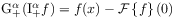
[42.3.6] If ![]() is the infinitesimal generator of a
is the infinitesimal generator of a
[page 43, §0]
semigroup
![]() (see Section 2.3.3.2 for definitions of
(see Section 2.3.3.2 for definitions of ![]() and
and ![]() ) on a Banach space
) on a Banach space ![]() then its fractional power is defined as
then its fractional power is defined as
![(-\mathrm{A})^{\alpha}f=\lim _{{\varepsilon\to 0+}}\frac{1}{-\Gamma(-\alpha)}\int\limits _{\varepsilon}^{\infty}t^{{-\alpha-1}}[\mathbf{1}-T(t)]f\mathrm{d}t](mi/mi84.png) |
(2.125) |
for every ![]() for which the limit exists in the norm
of
for which the limit exists in the norm
of ![]() [120, 121, 93, 123].
[43.0.1] This aproach is clearly inspired by the Marchaud form (2.82).
Alternatively, one may use the Grünwald approach
to define fractional powers of semigroup generators [122, 99].
[120, 121, 93, 123].
[43.0.1] This aproach is clearly inspired by the Marchaud form (2.82).
Alternatively, one may use the Grünwald approach
to define fractional powers of semigroup generators [122, 99].
2.2.2.10 Pseudodifferential Operators
[43.1.1] The calculus of pseudodifferential operators represents another generalization of the operator calculus in Hilbert spaces. [43.1.2] It has its roots in Hadamard’s ideas [36], Riesz potentials [97], Feller’s suggestion [26] and Calderon-Zygmund singular integrals [16]. [43.1.3] Later it was generalized and became a tool for treating elliptic partial differential operators with nonconstant coefficients.
Definition 2.19
[43.2.1] A (Kohn-Nirenberg) pseudodifferential operator of order ![]()
![]() is defined as
is defined as
| (2.126) |
and the function ![]() is called its symbol.
[43.2.2] The symbol is in the Kohn-Nirenberg symbol class
is called its symbol.
[43.2.2] The symbol is in the Kohn-Nirenberg symbol class ![]() if it is in
if it is in ![]() , and there exists a
compact set
, and there exists a
compact set ![]() such that
such that
![]() , and for any pair
of multiindices
, and for any pair
of multiindices ![]() there is a constant
there is a constant ![]() such
that
such
that
| (2.127) |
[43.2.3] The Hörmander symbol class ![]() is obtained by
replacing the exponent
is obtained by
replacing the exponent ![]() on the right hand side
with
on the right hand side
with ![]() where
where ![]() .
.
[43.3.1] Pseudodifferential operators provide a unified approach to differential and integral or convolution operators that are ‘‘nearly’’ translation invariant. [43.3.2] They have a close relation with Weyl quantization in physics [116, 28]. However, they will not be discussed further because the traditional symbol classes do not contain the usual fractional derivative operators. [43.3.3] Fractional Riesz derivatives are not pseudodifferential operators in the sense above. [43.3.4] Their symbols do not fall into any of the standard Kohn-Nirenberg or Hörmander symbol classes due to lack of differentiability at the origin.
[page 44, §1]
2.2.3 Eigenfunctions
[44.1.1] The eigenfunctions of Riemann-Liouville fractional derivatives are defined as the solutions of the fractional differential equation
| (2.128) |
where ![]() is the eigenvalue.
[44.1.2] They are readily identifed using eq. (A.11)
as
is the eigenvalue.
[44.1.2] They are readily identifed using eq. (A.11)
as
| (2.129) |
where
| (2.130) |
is the generalized Mittag-Leffler function [125, 126].
[44.1.3] More generally the eigenvalue equation for
fractional derivatives of order ![]() and type
and type ![]() reads
reads
| (2.131) |
and it is solved by [54, eq.124]
| (2.132) |
[page 45, §0]
where the case ![]() corresponds to (2.128).
[45.0.1] A second important special case is the equation
corresponds to (2.128).
[45.0.1] A second important special case is the equation
| (2.133) |
with ![]() .
[45.0.2] In this case the eigenfunction
.
[45.0.2] In this case the eigenfunction
| (2.134) |
where ![]() is the Mittag-Leffler function
[86].
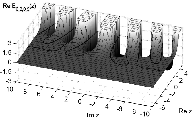
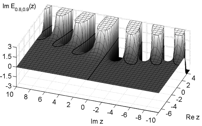
[45.0.3] The Mittag-Leffler function plays a central role
in fractional calculus.
[45.0.4] It has only recently been calculated numerically
in the full complex plane
[108, 62].
[45.0.5] Figure 2.1 and 2.2
illustrate
is the Mittag-Leffler function
[86].
[45.0.3] The Mittag-Leffler function plays a central role
in fractional calculus.
[45.0.4] It has only recently been calculated numerically
in the full complex plane
[108, 62].
[45.0.5] Figure 2.1 and 2.2
illustrate ![]() for a rectangular region in the
complex plane (see [108]).
[45.1.1] The solid line in Figure 2.1 is the line
for a rectangular region in the
complex plane (see [108]).
[45.1.1] The solid line in Figure 2.1 is the line
![]() , in Figure 2.2 it
is
, in Figure 2.2 it
is ![]() .
.
[45.2.1] Note, that some authors are avoiding the operator
![]() in fractional differential equations
(see e.g. [112, 101, 84, 111, 7, 82]
or chapters in this volume).
[45.2.2] In their notation the eigenvalue equation
(2.133) becomes (c.f.[112, eq.(22)])
in fractional differential equations
(see e.g. [112, 101, 84, 111, 7, 82]
or chapters in this volume).
[45.2.2] In their notation the eigenvalue equation
(2.133) becomes (c.f.[112, eq.(22)])
| (2.135) |
containing two derivative operators instead of one.
