4 Identification of capillary pressure

4.1 Hydrostatic equilibrium

[5.0.1.1] The constitutive theory proposed above, contrary to the traditional theory, does not postulate a unique capillary pressure as a constitutive parameter function. [5.0.1.2] On the other hand experimental evidence suggests that capillary pressure is a useful concept to correlate observations. [5.0.1.3] To make contact with the established traditional theory it is therefore important to check whether the traditional $P_{{\rm c}}({S_{{\mathbb{W}}}})$ relation can be viewed as a derived concept within the new theory.

[5.0.2.1] Consider first the case of hydrostatic equilibrium where ${\mathbf{v}}_{i}=0$ for all $i=1,2,3,4$ . [5.0.2.2] In hydrostatic equilibrium all fluids are at rest. [5.0.2.3] In this case the traditional theory implies $\partial{S_{{\mathbb{W}}}}/\partial t=0$ and $\partial{S_{{\mathbb{O}}}}/\partial t=0$ , by mass balance eq. (11). [5.0.2.4] The traditional momentum balance eqs. (12) can be integrated to give

$\displaystyle{P_{{\mathbb{W}}}}(\mathbf{x})$	$\displaystyle={P_{{\mathbb{W}}}}(\mathbf{x}_{0})+\varrho _{{\mathbb{W}}}\mathbf{g}\cdot(\mathbf{x}-\mathbf{x}_{0})$		(31a)
$\displaystyle{P_{{\mathbb{O}}}}(\mathbf{x})$	$\displaystyle={P_{{\mathbb{O}}}}(\mathbf{x}_{0})+\varrho _{{\mathbb{O}}}\mathbf{g}\cdot(\mathbf{x}-\mathbf{x}_{0})$		(31b)

where $\mathbf{x}_{0}$ is a point in the boundary. [5.0.2.5] Combined with the assumption (13) one finds

$\displaystyle P_{{\rm c}}({S_{{\mathbb{W}}}}(\mathbf{x}))$	$\displaystyle={P_{{\mathbb{O}}}}(\mathbf{x})-{P_{{\mathbb{W}}}}(\mathbf{x})$		(32)
	$\displaystyle=P_{{\rm c0}}+(\varrho _{{\mathbb{O}}}-\varrho _{{\mathbb{W}}})\mathbf{g}\cdot(\mathbf{x}-\mathbf{x}_{0})$

implying the existence of a unique hydrostatic saturation profile ${S_{{\mathbb{W}}}}(\mathbf{x})$ . [5.0.2.6] Here $P_{{\rm c0}}=P_{{\rm c}}(\mathbf{x}_{0})$ is the capillary pressure at $\mathbf{x}=\mathbf{x}_{0}$ . [5.0.2.7] Experiments show, however, that hydrostatic saturation profiles are not unique. [5.0.2.8] As a consequence the traditional theory employs multiple $P_{{\rm c}}({S_{{\mathbb{W}}}})$ relations for drainage and imbibition, and this leads to difficult problems when imbibition and drainage occur simultaneously.

[5.0.3.1] The nonlinear theory proposed here can be solved in the special case of hydrostatic equilibrium. [5.0.3.2] Mass balance (1) now implies $\partial S_{i}/\partial t=0$ for all $i=1,2,3,4$ . [5.0.3.3] Integrating eqs. (2) yields

$\displaystyle P_{1}(\mathbf{x})$	$\displaystyle=P_{1}(\mathbf{x}_{0})+\varrho _{{\mathbb{W}}}\mathbf{g}\cdot(\mathbf{x}-\mathbf{x}_{0})$	(33a)
$\displaystyle P_{3}(\mathbf{x})$	$\displaystyle=P_{3}(\mathbf{x}_{0})+\Pi _{{\rm a}}\left(S_{1}(\mathbf{x})^{{-\alpha}}-S_{1}(\mathbf{x}_{0})^{{-\alpha}}\right)$	(33b)
	$\displaystyle+\gamma P^{*}_{2}\left(S_{2}(\mathbf{x})^{{\gamma-1}}-S_{2}(\mathbf{x}_{0})^{{\gamma-1}}\right)$
	$\displaystyle+\varrho _{{\mathbb{W}}}\mathbf{g}\cdot(\mathbf{x}-\mathbf{x}_{0})$
$\displaystyle P_{3}(\mathbf{x})$	$\displaystyle=P_{3}(\mathbf{x}_{0})+\varrho _{{\mathbb{O}}}\mathbf{g}\cdot(\mathbf{x}-\mathbf{x}_{0})$	(33c)
$\displaystyle P_{1}(\mathbf{x})$	$\displaystyle=P_{1}(\mathbf{x}_{0})+\Pi _{{\rm b}}\left(S_{3}(\mathbf{x})^{{-\beta}}-S_{3}(\mathbf{x}_{0})^{{-\beta}}\right)$	(33d)
	$\displaystyle+\delta P^{*}_{4}\left(S_{4}(\mathbf{x})^{{\delta-1}}-S_{4}(\mathbf{x}_{0})^{{\delta-1}}\right)$
	$\displaystyle+\varrho _{{\mathbb{O}}}\mathbf{g}\cdot(\mathbf{x}-\mathbf{x}_{0})$

If one identifies $P_{1}$ with ${P_{{\mathbb{W}}}}$ and $P_{3}$ with ${P_{{\mathbb{O}}}}$ then eqs. (33a) and (33b) suggest to identify $P_{{\rm c}}$ as $P_{3}-P_{1}$ . [5.1.0.1] Then eqs. (33c) and (33d) combined with $S_{1}={S_{{\mathbb{W}}}}-S_{2}$ and $S_{3}=1-{S_{{\mathbb{W}}}}-S_{4}$ imply $P_{{\rm c}}=P_{{\rm c}}({S_{{\mathbb{W}}}},S_{2},S_{4})$ . [5.1.0.2] The capillary pressure $P_{{\rm c}}$ depends not only on ${S_{{\mathbb{W}}}}$ but also on $S_{2}$ and $S_{4}$ in hydrostatic equilibrium. [5.1.0.3] In the theory proposed here it is not possible to identify a unique $P_{{\rm c}}({S_{{\mathbb{W}}}})$ relation when all fluids are at rest. This agrees with experiment.

4.2 Residual decoupling approximation

[5.1.1.1] While it is not possible to identify a unique $P_{{\rm c}}({S_{{\mathbb{W}}}})$ relation in hydrostatic equilibrium such a functional relation emerges nevertheless from the present theory when the system approaches hydrostatic equilibrium in the residual decoupling approximation. [5.1.1.2] The approach to hydrostatic equilibrium in the residual decoupling approximation (RDA) can be formulated mathematically as ${\mathbf{v}}_{4}=\mathbf{0},{\mathbf{v}}_{2}=\mathbf{0}$ and $R_{{23}}=0,R_{{41}}=0$ . [5.1.1.3] In addition it is assumed that the velocities ${\mathbf{v}}_{1},{\mathbf{v}}_{3}\to 0$ are small but nonzero. [5.1.1.4] In the RDA mass balance becomes

$\displaystyle\frac{\partial S_{1}}{\partial t}$	$\displaystyle+\mathbf{\nabla}\cdot(S_{1}{\mathbf{v}}_{1})={\eta _{{2}}}\left(\frac{S_{2}-{{S_{2}}^{}}}{{{S_{{\mathbb{W}}}}^{}}-{S_{{\mathbb{W}}}}}\right)\frac{\partial{S_{{\mathbb{W}}}}}{\partial t}$	(34a)
$\displaystyle\frac{\partial S_{2}}{\partial t}$	$\displaystyle=-{\eta _{{2}}}\left(\frac{S_{2}-{{S_{2}}^{}}}{{{S_{{\mathbb{W}}}}^{}}-{S_{{\mathbb{W}}}}}\right)\frac{\partial{S_{{\mathbb{W}}}}}{\partial t}$	(34b)
$\displaystyle\frac{\partial S_{3}}{\partial t}$	$\displaystyle+\mathbf{\nabla}\cdot(S_{3}{\mathbf{v}}_{3})={\eta _{{4}}}\left(\frac{S_{4}-{{S_{4}}^{}}}{{{S_{{\mathbb{O}}}}^{}}-{S_{{\mathbb{O}}}}}\right)\frac{\partial{S_{{\mathbb{O}}}}}{\partial t}$	(34c)
$\displaystyle\frac{\partial S_{4}}{\partial t}$	$\displaystyle=-{\eta _{{4}}}\left(\frac{S_{4}-{{S_{4}}^{}}}{{{S_{{\mathbb{O}}}}^{}}-{S_{{\mathbb{O}}}}}\right)\frac{\partial{S_{{\mathbb{O}}}}}{\partial t}$	(34d)

Momentum balance becomes in the RDA

	$\displaystyle\phi _{1}(\mathbf{\nabla}P_{1}-\varrho _{{\mathbb{W}}}\mathbf{g})=R_{{13}}{\mathbf{v}}_{3}-(R_{1}+M_{1}){\mathbf{v}}_{1}$		(35a)
	$\displaystyle 0=\phi _{2}(\mathbf{\nabla}P_{3}+\mathbf{\nabla}{\Pi _{c}}_{{\mathbb{W}}}-\gamma P^{*}_{2}\mathbf{\nabla}S_{2}^{{\gamma-1}}-\varrho _{{\mathbb{W}}}\mathbf{g})$		(35b)
	$\displaystyle\phi _{3}(\mathbf{\nabla}P_{3}-\varrho _{{\mathbb{O}}}\mathbf{g})=R_{{31}}{\mathbf{v}}_{1}-(R_{3}+M_{3}){\mathbf{v}}_{3}$		(35c)
	$\displaystyle 0=\phi _{4}(\mathbf{\nabla}P_{1}+\mathbf{\nabla}{\Pi _{c}}_{{\mathbb{O}}}-\delta P^{*}_{4}\mathbf{\nabla}S_{4}^{{\delta-1}}-\varrho _{{\mathbb{O}}}\mathbf{g})$		(35d)

where the abbreviations

$\displaystyle R_{1}$	$\displaystyle=R_{{13}}+R_{{14}}+R_{{15}}$		(36a)
$\displaystyle R_{3}$	$\displaystyle=R_{{31}}+R_{{32}}+R_{{35}}$		(36b)

were used. [5.1.1.5] Equations (34) and (35) together with eq.(16b) provide 17 equations for 12 variables ( $P_{1},P_{3},{\mathbf{v}}_{1},{\mathbf{v}}_{3}$ and $S_{i},i=1,2,3,4$ ).

[5.1.2.1] Equations (34) and (35) can now be compared to the traditional equations (11)–(13) with the aim of identifying capillary pressure and relative permeability. [5.1.2.2] Consider first the momentum balance eqs. (35). [5.1.2.3] As in the traditional theory [24] viscous decoupling is assumed to hold, i.e. $R_{{31}}=0$ and $R_{{13}}=0$ . [5.1.2.4] Next, assuming that $R_{1}\gg M_{1}$ , $R_{3}\gg M_{3}$ , and $S_{i}\neq 0$ one finds [page 6, §0]

	$\displaystyle\phi _{1}(\mathbf{\nabla}P_{1}-\varrho _{{\mathbb{W}}}\mathbf{g})=-R_{1}{\mathbf{v}}_{1}=-R_{1}\frac{\phi _{{\mathbb{W}}}}{\phi _{1}}{\mathbf{v}}_{{\mathbb{W}}}$		(37a)
	$\displaystyle\mathbf{\nabla}P_{3}=-\mathbf{\nabla}{\Pi _{c}}_{{\mathbb{W}}}+\gamma P^{*}_{2}\mathbf{\nabla}S_{2}^{{\gamma-1}}+\varrho _{{\mathbb{W}}}\mathbf{g}$		(37b)
	$\displaystyle\phi _{3}(\mathbf{\nabla}P_{3}-\varrho _{{\mathbb{O}}}\mathbf{g})=-R_{3}{\mathbf{v}}_{3}=-R_{3}\frac{\phi _{{\mathbb{O}}}}{\phi _{3}}{\mathbf{v}}_{{\mathbb{O}}}$		(37c)
	$\displaystyle\mathbf{\nabla}P_{1}=-\mathbf{\nabla}{\Pi _{c}}_{{\mathbb{O}}}+\delta P^{*}_{4}\mathbf{\nabla}S_{4}^{{\delta-1}}+\varrho _{{\mathbb{O}}}\mathbf{g}$		(37d)

where barycentric velocities ${\mathbf{v}}_{{\mathbb{W}}},{\mathbf{v}}_{{\mathbb{O}}}$ defined through

$\displaystyle{S_{{\mathbb{W}}}}{\mathbf{v}}_{{\mathbb{W}}}$	$\displaystyle=S_{1}{\mathbf{v}}_{1}+S_{2}{\mathbf{v}}_{2}$		(38a)
$\displaystyle{S_{{\mathbb{O}}}}{\mathbf{v}}_{{\mathbb{O}}}$	$\displaystyle=S_{3}{\mathbf{v}}_{3}+S_{4}{\mathbf{v}}_{4}$		(38b)

have been introduced. [6.0.0.1] Subtracting eq. (37a) from eq. (37c), as well as eq. (37d) from eq. (37b), and equating the result gives

	$\displaystyle 2(\varrho _{{\mathbb{O}}}-\varrho _{{\mathbb{W}}})\mathbf{g}+\frac{R_{1}}{\phi _{1}^{2}}\phi _{{\mathbb{W}}}{\mathbf{v}}_{{\mathbb{W}}}-\frac{R_{3}}{\phi _{3}^{2}}\phi _{{\mathbb{O}}}{\mathbf{v}}_{{\mathbb{O}}}=$
	$\displaystyle\mathbf{\nabla}\left(\Pi _{{\rm a}}S_{1}^{{-\alpha}}-\Pi _{{\rm b}}S_{3}^{{-\beta}}+\gamma P^{}_{2}S_{2}^{{\gamma-1}}-\delta P^{}_{4}S_{4}^{{\delta-1}}\right)$		(39)

where eq. (22) has also been employed. [6.0.0.2] This result can be compared to the traditional theory where one finds from eqs. (12) and (13)

$(\varrho _{{\mathbb{O}}}-\varrho _{{\mathbb{W}}})\mathbf{g}+\frac{\mu _{{\mathbb{W}}}}{kk^{r}_{{\mathbb{W}}}}\phi _{{\mathbb{W}}}{\mathbf{v}}_{{\mathbb{W}}}-\frac{\mu _{{\mathbb{O}}}}{kk^{r}_{{\mathbb{O}}}}\phi _{{\mathbb{O}}}{\mathbf{v}}_{{\mathbb{O}}}=\mathbf{\nabla}P_{{\rm c}}$

(40)

Again this seems to imply $P_{{\rm c}}=P_{{\rm c}}({S_{{\mathbb{W}}}},S_{2},S_{4})$ as already found above for hydrostatic equilibrium. [6.0.0.3] However, within the RDA additional constraints follow from mass balance (34).

[6.0.1.1] First, observe that adding (34a) to (34b) resp. (34c) to (34d) with the help of eq. (38a) yields the traditional mass balance eqs. (11). [6.0.1.2] Next, verify by insertion that eqs. (34b) and (34d) admit the solutions

$\displaystyle S_{2}(\mathbf{x},t)$	$\displaystyle={{S_{2}}^{}}(\mathbf{x})+(S_{{20}}(\mathbf{x})-{{S_{2}}^{}}(\mathbf{x}))$	(41a)
	$\displaystyle\times\left(\frac{{{S_{{\mathbb{W}}}}^{}}(\mathbf{x})-{S_{{\mathbb{W}}}}(\mathbf{x},t)}{{{S_{{\mathbb{W}}}}^{}}(\mathbf{x})-{S_{{\mathbb{W}0}}}(\mathbf{x})}\right)^{{\eta _{{2}}}}$
$\displaystyle S_{4}(\mathbf{x},t)$	$\displaystyle={{S_{4}}^{}}(\mathbf{x})+(S_{{40}}(\mathbf{x})-{{S_{4}}^{}}(\mathbf{x}))$	(41b)
	$\displaystyle\times\left(\frac{{S_{{\mathbb{W}}}}(\mathbf{x},t)-{{S_{{\mathbb{W}}}}^{}}(\mathbf{x})}{{S_{{\mathbb{W}0}}}(\mathbf{x})-{{S_{{\mathbb{W}}}}^{}}(\mathbf{x})}\right)^{{\eta _{{4}}}}$

where the displacement process is assumed to start from the initial conditions

$\displaystyle{S_{{\mathbb{W}}}}(\mathbf{x},t_{0})$	$\displaystyle={S_{{\mathbb{W}0}}}(\mathbf{x})$	(42a)
$\displaystyle S_{2}(\mathbf{x},t_{0})$	$\displaystyle=S_{{20}}(\mathbf{x})$	(42b)
$\displaystyle S_{4}(\mathbf{x},t_{0})$	$\displaystyle=S_{{40}}(\mathbf{x})$	(42c)

at some initial instant $t_{0}$ . [6.1.0.1] The limiting saturations ${{S_{{\mathbb{W}}}}^{*}}$ , ${{S_{{\mathbb{O}}}}^{*}}$ , ${{S_{2}}^{*}},{{S_{4}}^{*}}$ are given by eqs. (29). [6.1.0.2] They depend only on the sign of $\partial{S_{{\mathbb{W}}}}/\partial t$ if $\tau\gg\partial{S_{{\mathbb{W}}}}/\partial t$ can be assumed to hold. [6.1.0.3] One finds in this case

$\displaystyle{{S_{{\mathbb{W}}}}^{*}}$	$\displaystyle=1-S_{{\mathbb{O}\,\rm im}}$	(43a)
$\displaystyle{{S_{{\mathbb{O}}}}^{*}}$	$\displaystyle=S_{{\mathbb{O}\,\rm im}}$	(43b)
$\displaystyle{{S_{2}}^{*}}$	$\displaystyle=0$	(43c)
$\displaystyle{{S_{4}}^{*}}$	$\displaystyle=S_{{\mathbb{O}\,\rm im}}$	(43d)

for imbibition processes (i.e. $\partial{S_{{\mathbb{W}}}}/\partial t>0$ ), resp.

$\displaystyle{{S_{{\mathbb{W}}}}^{*}}$	$\displaystyle=S_{{\mathbb{W}\,\rm dr}}$	(44a)
$\displaystyle{{S_{{\mathbb{O}}}}^{*}}$	$\displaystyle=1-S_{{\mathbb{W}\,\rm dr}}$	(44b)
$\displaystyle{{S_{2}}^{*}}$	$\displaystyle=S_{{\mathbb{W}\,\rm dr}}$	(44c)
$\displaystyle{{S_{4}}^{*}}$	$\displaystyle=0$	(44d)

for drainage processes (i.e. $\partial{S_{{\mathbb{W}}}}/\partial t<0$ ).

[6.1.1.1] With these solutions in hand the capillary pressure can be identified up to a constant as

	$\displaystyle P_{{\rm c}}({S_{{\mathbb{W}}}})=\frac{1}{2}\left[\Pi _{{\rm a}}({S_{{\mathbb{W}}}}-S_{2})^{{-\alpha}}\right.$		(45)
	$\displaystyle\left.-\Pi _{{\rm b}}(1-{S_{{\mathbb{W}}}}-S_{4})^{{-\beta}}+\gamma P^{}_{2}S_{2}^{{\gamma-1}}-\delta P^{}_{4}S_{4}^{{\delta-1}}\right]$

where $S_{2}=S_{2}({S_{{\mathbb{W}}}})$ and $S_{4}=S_{4}({S_{{\mathbb{W}}}})$ are given by eqs. (41). [6.1.1.2] This result holds in the RDA combined with the assumptions above. [6.1.1.3] Furthermore, equations (37a) and (37c) are recognized as generalized Darcy laws with relative permeabilities identified as

$\displaystyle k^{r}_{{\mathbb{W}}}({S_{{\mathbb{W}}}})$	$\displaystyle=2R_{1}^{{-1}}\frac{\mu _{{\mathbb{W}}}}{k}\phi^{2}({S_{{\mathbb{W}}}}-S_{2})^{2}$		(46a)
$\displaystyle k^{r}_{{\mathbb{O}}}({S_{{\mathbb{W}}}})$	$\displaystyle=2R_{3}^{{-1}}\frac{\mu _{{\mathbb{O}}}}{k}\phi^{2}(1-{S_{{\mathbb{W}}}}-S_{4})^{2}$		(46b)

where $S_{2}=S_{2}({S_{{\mathbb{W}}}})$ and $S_{4}=S_{4}({S_{{\mathbb{W}}}})$ are again given by eqs. (41).

Figure 1: Hysteresis loop and drainage scanning curves for capillary pressure $P_{{\rm c}}$ as function of water saturation ${S_{{\mathbb{W}}}}$ fitted to experimental data obtained for a water wet medium grained sand of porosity $\phi=0.34$ . The primary drainage curve is the dash-dotted line. The main hysteresis loop is the solid line. The dashed lines are drainage scanning curves. All eight curves have the same parameters: $S_{{\mathbb{W}\,\rm dr}}=0.15$ , $S_{{\mathbb{O}\,\rm im}}=0.19$ , $\alpha=0.52$ , $\beta=0.90$ , $\gamma=1.5$ , $\delta=3.5$ ${\eta _{{2}}}=4$ , ${\eta _{{4}}}=3$ , $\Pi _{{\rm a}}=1620$ Pa, $\Pi _{{\rm b}}=25$ Pa, and $P^{*}_{2}=2500$ Pa $P^{*}_{4}=400$ Pa. The five scanning curves start from the boundary imbibition curve at ${S_{{\mathbb{W}}}}=0.3,0.4,0.5,0.6,0.7$ .

Figure 2: Hysteresis loop for capillary pressure $P_{{\rm c}}$ as function of water saturation ${S_{{\mathbb{W}}}}$ as in Fig. 1. The imbibition scanning curves start from the secondary drainage curve. Parameters and line styles are identical to those in Figure 1.

4.3 Reproduction of experimental observations

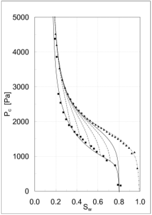
[6.1.2.1] Figure 1 visualizes the results obtained by fitting eq. (45) to experiment. [6.1.2.2] The experimental results are depicted as triangles (primary drainage) and squares (imbibition). [6.1.2.3] The experiments were performed in a medium grained unconsolidated water wet sand of porosity $\phi=0.34$ . [6.1.2.4] Water was used as wetting fluid while air resp. TCE were used as the nonwetting fluid. [6.1.2.5] The experiments were carried out over a period of several weeks at the Versuchseinrichtung zur Grundwasser- und Altlastensanierung (VEGAS) [page 7, §0] at the Universität Stuttgart. [7.0.0.1] They are described in more detail in Ref. [25]. The parameters for all the curves shown in all four figures are $S_{{\mathbb{W}\,\rm dr}}=0.15$ , $S_{{\mathbb{O}\,\rm im}}=0.19$ , $\alpha=0.52$ , $\beta=0.90$ , $\gamma=1.5$ , $\delta=3.5$ ${\eta _{{2}}}=4$ , ${\eta _{{4}}}=3$ , $\Pi _{{\rm a}}=1620$ Pa, $\Pi _{{\rm b}}=25$ Pa, and $P^{*}_{2}=2500$ Pa $P^{*}_{4}=400$ Pa.

[7.0.1.1] If it is further assumed that the medium is isotropic and that the matrices $R_{1},R_{3}$ have the form

$\displaystyle R_{1}$	$\displaystyle=R^{*}_{1}\phi _{1}^{{-{\kappa _{\mathbb{W}}}}}\mathbf{1}$		(47a)
$\displaystyle R_{3}$	$\displaystyle=R^{*}_{3}\phi _{3}^{{-{\kappa _{\mathbb{O}}}}}\mathbf{1}$		(47b)

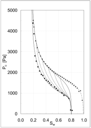
then the relative permeability functions are obtained from eqs. (46). [7.0.1.2] The result for the special case ${\kappa _{\mathbb{W}}}={\kappa _{\mathbb{O}}}=0$ is shown in Figures 3 and 4. [7.0.1.3] The parameters $R^{*}_{1},R^{*}_{3}$ are chosen such that $R^{*}_{1}=2\phi^{2}\mu _{{\mathbb{W}}}/k$ and $R^{*}_{3}=2\phi^{2}\mu _{{\mathbb{O}}}/k$ , where $\mu _{{\mathbb{W}}},\mu _{{\mathbb{O}}}$ are the fluid viscosities and $k$ is the absolute permeability of the medium. [7.0.1.4] All other parameters for the relative permeability functions shown in Figures 3 and 4 are identical to those of the capillary pressure curves in Figures 1 and 2.

Figure 3: Hysteresis loop and drainage scanning curves for relative permeabilities $k^{r}_{{\mathbb{W}}},k^{r}_{{\mathbb{O}}}$ as function of water saturation ${S_{{\mathbb{W}}}}$ . Parameters and line styles are identical to those for capillary pressure in Figures 1 and 2. Here ${\kappa _{\mathbb{W}}}={\kappa _{\mathbb{O}}}=0$ and the parameters $R^{*}_{1},R^{*}_{3}$ are chosen such that $R^{*}_{1}=2\phi^{2}\mu _{{\mathbb{W}}}/k$ and $R^{*}_{3}=2\phi^{2}\mu _{{\mathbb{O}}}/k$ .

Figure 4: Same as Figure 3 with imbibition scanning curves starting from the secondary drainage curve. Parameters and line styles are identical to those in Figure 3.

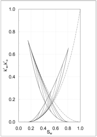
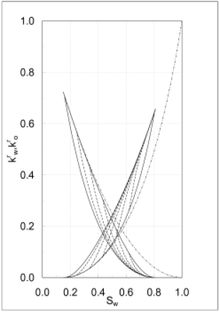
[7.0.2.1] Note that Figures 1 through 4 show a total of 30 different scanning curves, 5 drainage and 5 imbibition scanning curves each for $P_{{\rm c}},k^{r}_{{\mathbb{W}}}$ and $k^{r}_{{\mathbb{O}}}$ . [7.1.0.1] In addition a total of 9 different bounding curves are displayed, namely the primary drainage, secondary drainage and secondary imbibition curve for $P_{{\rm c}},k^{r}_{{\mathbb{W}}}$ and $k^{r}_{{\mathbb{O}}}$ . [7.1.0.2] Three more bounding curves namely primary imbibition for $P_{{\rm c}},k^{r}_{{\mathbb{W}}}$ and $k^{r}_{{\mathbb{O}}}$ starting from ${S_{{\mathbb{W}}}}=0$ are not shown because they are difficult to obtain experimentally for a water-wet sample. [7.1.0.3] Of course the number of scanning curves can be increased indefinitely. [7.1.0.4] All of these curves have the same values of the constitutive parameters. [7.1.0.5] There is less than one parameter per curve. [7.1.0.6] The curves shown in the figures exhibit the full range of hysteretic phenomena known from experiment. [7.1.0.7] Nevertheless it should be kept in mind that these curves are obtained only under special approximations, and when these are not valid such curves do not exist.

Author:	R. Hilfer
originally published in:	Physical Review E 73, 016307 (2006)
originally submitted:	20. 05. 2005