5 Results
[190.1.1] The results for ![]() will be expressed via the so called correlation factor
will be expressed via the so called correlation factor ![]() .
[190.1.2] It is a measure which is often used to characterize the amount
by which the self diffusion coefficient of a tracer particle in a lattice gas
differs from its mean field value given by the vacancy concentration.
[190.1.3] All results will be presented and discussed with the conventions
.
[190.1.2] It is a measure which is often used to characterize the amount
by which the self diffusion coefficient of a tracer particle in a lattice gas
differs from its mean field value given by the vacancy concentration.
[190.1.3] All results will be presented and discussed with the conventions ![]() ,
,
![]() , and assuming a unit lattice constant.
[190.1.4] In these dimensionless units
, and assuming a unit lattice constant.
[190.1.4] In these dimensionless units ![]() is defined by the equation
is defined by the equation ![]() or, more generally,
or, more generally,
| (5.1) |
because for our hopping models ![]() .
[190.1.5] In the limit
.
[190.1.5] In the limit ![]() exact results for the correlation factor
are known for the case
exact results for the correlation factor
are known for the case ![]() (and
(and ![]() )[11, 13, 14].
[page 191, §0]
[191.0.1] For the hexagonal lattice one has
)[11, 13, 14].
[page 191, §0]
[191.0.1] For the hexagonal lattice one has ![]() ,
while
,
while ![]() for the fcc lattice.
[191.0.2] These values will be used below to determine
for the fcc lattice.
[191.0.2] These values will be used below to determine ![]() in eq. (4.2).
in eq. (4.2).
[191.1.1] We now have to solve eq. (3.10) in conjunction with eqs. (3.13) and (4.4) for the cases of interest, the hexagonal and face centered cubic lattice. [191.1.2] The lattice Greens functions for these situations are well known and can be expressed in terms of the complete elliptic integral of the first kind
| (5.2) |
[191.1.3] For the hexagonal lattice we have
| (5.3) |
For the fcc lattice the Greens function is given by
| (5.4) |
where
| (5.5) |
[191.1.4] We now solve eq. (3.10) iteratively on the computer.
[191.1.5] We stop the iteration when the maximal relative error
between two consecutive solutions falls below ![]() .
[191.1.6] The resulting
.
[191.1.6] The resulting ![]() is then used to calculate
is then used to calculate ![]() according to eqs. (3.13) and (4.4).
[191.1.7] The results are displayed in Figures 2 through 10.
according to eqs. (3.13) and (4.4).
[191.1.7] The results are displayed in Figures 2 through 10.
[191.2.1] First we determine the proportionality constant ![]() in eq. (4.2).
[191.2.2] This is achieved by requiring that the calculated correlation factor
reproduces the known exact results for the limit
in eq. (4.2).
[191.2.2] This is achieved by requiring that the calculated correlation factor
reproduces the known exact results for the limit ![]() .
[191.2.3] We find
.
[191.2.3] We find ![]() for the hexagonal lattice,
and
for the hexagonal lattice,
and ![]() for the fcc lattice.
[191.2.4] These numbers are difficult to determine numerically,
and we estimate the error to be roughly
for the fcc lattice.
[191.2.4] These numbers are difficult to determine numerically,
and we estimate the error to be roughly ![]() .
[191.2.5] In all subsequent calculations we then use these values for
.
[191.2.5] In all subsequent calculations we then use these values for ![]() .
.
[page 193, §1]
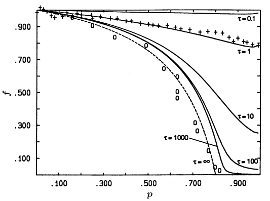
[193.1.1] In Figure 2 we have extracted the correlation factor from ![]() and plotted it versus blocker concentration
and plotted it versus blocker concentration ![]() .
[193.1.2] All curves are for the uncorrelated case,
i. e.
.
[193.1.2] All curves are for the uncorrelated case,
i. e. ![]() , on the fcc lattice.
[193.1.3] We give results for
, on the fcc lattice.
[193.1.3] We give results for ![]() and
and ![]() .
[193.1.4] The crosses are the results of the Monte Carlo simulation
for the case
.
[193.1.4] The crosses are the results of the Monte Carlo simulation
for the case ![]() taken from Ref. [7].
[193.1.5] The circles are MC-results for
taken from Ref. [7].
[193.1.5] The circles are MC-results for ![]() and were taken from Ref. [10].
[193.1.6] Clearly there will be a discrepancy for this case
because our results are approximate and for bond percolation
while the simulation is exact and for site percolation.
[193.1.7] An immediate problem is the value of
and were taken from Ref. [10].
[193.1.6] Clearly there will be a discrepancy for this case
because our results are approximate and for bond percolation
while the simulation is exact and for site percolation.
[193.1.7] An immediate problem is the value of ![]() for which the effective medium theory gives
for which the effective medium theory gives
![]() while the exact value is
while the exact value is ![]() [8].
[193.1.8] If we simply use the exact value for
[8].
[193.1.8] If we simply use the exact value for ![]() in our calculation
we obtain the dashed line displayed in Fig. 2
which is found to be in good agreement.
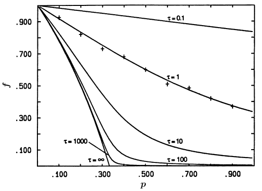
[193.1.9] In Fig. 3 we plot
in our calculation
we obtain the dashed line displayed in Fig. 2
which is found to be in good agreement.
[193.1.9] In Fig. 3 we plot ![]() vs.
vs. ![]() for the hexagonal lattice.
[193.1.10] Here the simulations have been taken from Ref. 10.
[193.1.11] Keeping in mind that there are no free parameters (remember
for the hexagonal lattice.
[193.1.10] Here the simulations have been taken from Ref. 10.
[193.1.11] Keeping in mind that there are no free parameters (remember ![]() )
we find very good agreement for both lattices.
[193.1.12] However, additional simulation data especially for
)
we find very good agreement for both lattices.
[193.1.12] However, additional simulation data especially for ![]() in the range
in the range ![]() , and a more accurate determination of
, and a more accurate determination of ![]() are required to fully evaluate the quality of the theoretical results.
[page 194, §0]
[194.0.1] We now turn to the results for our primary objective,
the frequency dependent diffusion coefficient.
are required to fully evaluate the quality of the theoretical results.
[page 194, §0]
[194.0.1] We now turn to the results for our primary objective,
the frequency dependent diffusion coefficient.
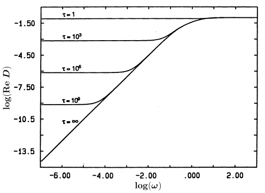
[194.1.1] We consider first the uncorrelated case ![]() on the fcc-lattice.
[194.1.2] In Figure 4 and Figure 5
we plot
on the fcc-lattice.
[194.1.2] In Figure 4 and Figure 5
we plot ![]() over ten decades in frequency on a log-log plot.
[194.1.3] Figure 4 corresponds to a blocker concentration
over ten decades in frequency on a log-log plot.
[194.1.3] Figure 4 corresponds to a blocker concentration ![]() which is below the percolation threshold for vacancies,
and shows the results for
which is below the percolation threshold for vacancies,
and shows the results for
![]() and
and ![]() .
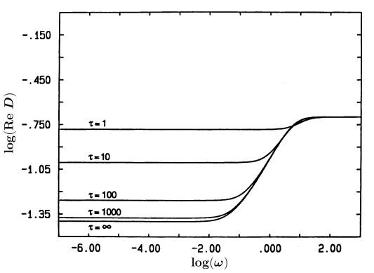
[194.1.4] Figure 5 has
.
[194.1.4] Figure 5 has ![]() and
and
![]() .
[194.1.5] From Figure 4 we see immediately that below the percolation threshold
.
[194.1.5] From Figure 4 we see immediately that below the percolation threshold ![]() vanishes quadratically with frequency for
vanishes quadratically with frequency for ![]() .
[194.1.6] This behaviour is well known from the analysis
of the EM theory for the frozen case.
[194.1.7] For
.
[194.1.6] This behaviour is well known from the analysis
of the EM theory for the frozen case.
[194.1.7] For ![]() we find a crossover to a constant proportional to
we find a crossover to a constant proportional to ![]() .
[194.1.8] This could have been expected because the blocker motion now allows the Aâparticle to get
through the network although the vacancy concentration at each instant is below
.
[194.1.8] This could have been expected because the blocker motion now allows the Aâparticle to get
through the network although the vacancy concentration at each instant is below ![]() .
[194.1.9] The mobility of the A-particles will be completely determined
by the mobility of the blockers.
[page 197, §0]
[197.0.1] The crossover frequency is seen to vary as
.
[194.1.9] The mobility of the A-particles will be completely determined
by the mobility of the blockers.
[page 197, §0]
[197.0.1] The crossover frequency is seen to vary as ![]() .
[197.0.2] This will be discussed further in the next section.
[197.0.3] On the other hand above the vacancy threshold Figure 5
shows that the effect of the blocker rearrangement is only noticeable
for
.
[197.0.2] This will be discussed further in the next section.
[197.0.3] On the other hand above the vacancy threshold Figure 5
shows that the effect of the blocker rearrangement is only noticeable
for ![]() values smaller than roughly
values smaller than roughly ![]() .
[197.0.4] Indeed one expects that the effect of blocker motion
will become negligible if
.
[197.0.4] Indeed one expects that the effect of blocker motion
will become negligible if ![]() is much smaler
than the d. c. conductivity in the frozen case
which is proportional to
is much smaler
than the d. c. conductivity in the frozen case
which is proportional to ![]() .
.
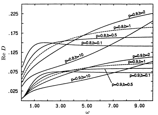
[197.1.1] In Figures 6 and 7 we now turn to the correlated case, i. e. ![]() .
[197.1.2] Again we consider the fcc-lattice and plot the real (Fig. 6)
and imaginary (Fig. 7) part of
.
[197.1.2] Again we consider the fcc-lattice and plot the real (Fig. 6)
and imaginary (Fig. 7) part of ![]() for the two concentrations
for the two concentrations ![]() and
and ![]() with fixed
with fixed ![]() but variable
but variable ![]() .
[197.1.3] We have chosen
.
[197.1.3] We have chosen ![]() for the correlation factor.
[197.1.4] The case
for the correlation factor.
[197.1.4] The case ![]() is included as a reference
and has been distinguished graphically by a dashed line.
[197.1.5] As before the real part approaches a constant as
is included as a reference
and has been distinguished graphically by a dashed line.
[197.1.5] As before the real part approaches a constant as ![]() irrespective of
irrespective of ![]() because
because ![]() is finite.
[197.1.6] A new phenomenon however is the appearance of nonmonotonous
behaviour for
is finite.
[197.1.6] A new phenomenon however is the appearance of nonmonotonous
behaviour for ![]() .
[197.1.7] In this case
.
[197.1.7] In this case ![]() is found to increase at low frequencies,
and to decrease at high frequencies
thereby exhibiting a maximum at a finite frequency.
[197.1.8] In general
is found to increase at low frequencies,
and to decrease at high frequencies
thereby exhibiting a maximum at a finite frequency.
[197.1.8] In general ![]() is found to decrease as
is found to decrease as ![]() at high frequencies,
and to increase at low frequencies.
[197.1.9] The reverse is seen for
at high frequencies,
and to increase at low frequencies.
[197.1.9] The reverse is seen for ![]() .
[197.1.10] This will also be discussed in the next section in more detail.
[197.1.11] For the imaginary part of
.
[197.1.10] This will also be discussed in the next section in more detail.
[197.1.11] For the imaginary part of ![]() we find a change of sign
for sufficiently small
we find a change of sign
for sufficiently small ![]() .
[197.1.12] See for example the case
.
[197.1.12] See for example the case ![]() ,
, ![]() .
[197.1.13] On the other hand for
.
[197.1.13] On the other hand for ![]() ,
, ![]() there is no change of sign in the imaginary part
while the real part still shows a maximum.
there is no change of sign in the imaginary part
while the real part still shows a maximum.
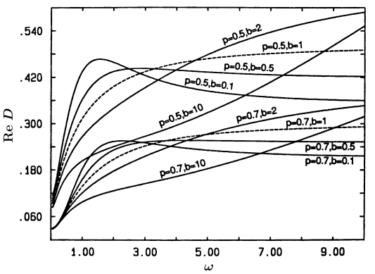
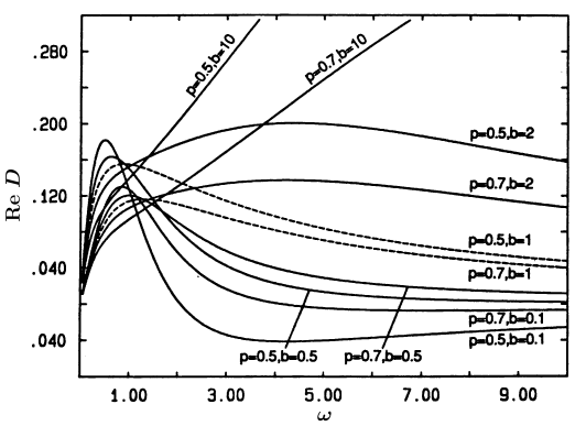
[197.2.1] The same calculations have been performed for the hexagonal lattice.
[197.2.2] The results are displayed in Figures 8 and 9.
[197.2.3] The only difference lies in the parameter values.
[197.2.4] We have chosen different concentrations, ![]() ,
, ![]() and fixed
and fixed ![]() at
at ![]() .
[197.2.5] The results show qualitatively the same behaviour as for the fcc-lattice.
.
[197.2.5] The results show qualitatively the same behaviour as for the fcc-lattice.
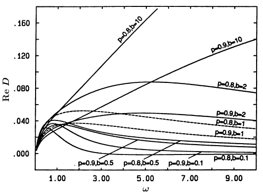
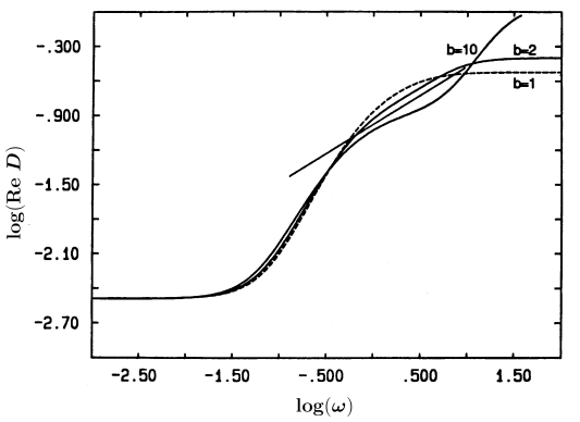
[197.3.1] In Figure 10 we have plotted some results
for the correlated case (![]() ) in a log-log plot.
[197.3.2] We show
) in a log-log plot.
[197.3.2] We show ![]() for
for ![]() ,
, ![]() and
and ![]() on the hexagonal lattice.
[197.3.3] We note that as a consequence of the correlations
the crossover into the constant high frequency limit
is smeared out and resembles a power law over more
than a decade in frequency.
[197.3.4] This is particularly apparent for the case
on the hexagonal lattice.
[197.3.3] We note that as a consequence of the correlations
the crossover into the constant high frequency limit
is smeared out and resembles a power law over more
than a decade in frequency.
[197.3.4] This is particularly apparent for the case ![]() .
.
[page 198, §0]
[198.1.1] For reference we have included a straight line into the graph
whose slope is found to be roughly ![]() .
[198.1.2] We remark that such a power law behaviour
for the frequency dependent conductivity
is often found experimentally in disordered systems.
[198.1.3] As a particular example we mention
.
[198.1.2] We remark that such a power law behaviour
for the frequency dependent conductivity
is often found experimentally in disordered systems.
[198.1.3] As a particular example we mention ![]() -
-![]() -alumina
where the ionic transport is also known to be highly correlated[34].
-alumina
where the ionic transport is also known to be highly correlated[34].
