1 Introduction
[page 89, §1]
[89.1.1] A large number of problems in theoretical physics,
including Schrödingers, Maxwell and Newtons
equations, can be formulated as initial value problems
for dynamical evolution equations of the form
| (1) |
where ![]() denotes time and B is an
operator on a Banach space.
[89.1.2] Depending on the initial data
denotes time and B is an
operator on a Banach space.
[89.1.2] Depending on the initial data ![]() describing
the state or observable of the system at time
describing
the state or observable of the system at time ![]() the problem
is to find the state or observable
the problem
is to find the state or observable ![]() of the system at later
times
of the system at later
times ![]() .
a (This is a footnote:) a
In classical mechanics the states are points in phase
space, the observables are functions on phase space,
and the operator B is specified by a vector field
and Poisson brackets.
In quantum mechanics (with finitely many degrees of
freedom) the states correspond to rays in a Hilbert
space, the observables to operators on this space,
and the operator B to the Hamiltonian.
In field theories the states are normalized positive
functionals on an algebra of operators or observables,
and then B becomes a derivation on the algebra
of observables.
The equations (1) need not be first order in time.
An example is the initial-value problem for the
wave equation for
.
a (This is a footnote:) a
In classical mechanics the states are points in phase
space, the observables are functions on phase space,
and the operator B is specified by a vector field
and Poisson brackets.
In quantum mechanics (with finitely many degrees of
freedom) the states correspond to rays in a Hilbert
space, the observables to operators on this space,
and the operator B to the Hamiltonian.
In field theories the states are normalized positive
functionals on an algebra of operators or observables,
and then B becomes a derivation on the algebra
of observables.
The equations (1) need not be first order in time.
An example is the initial-value problem for the
wave equation for ![]()
in one dimension.
It can be recast into the form of eq. (1)
by introducing a second variable
![]()
![]() and defining
and defining
![]()
[89.2.1] Many authors, mostly driven by the needs of applied problems, have considered generalizations of equation (1) of the form
| (2) |
in which the first order time derivative ![]() is replaced
with a certain fractional time derivative ‘‘
is replaced
with a certain fractional time derivative ‘‘![]() ’’
of order
’’
of order ![]() (see e.g.
[1]–[24]
and the Chapters IV–VIII in this book).
[89.2.2] A number of fundamental questions are raised by such a replacement.
[89.2.3] In order to appreciate these it is useful to recall that
the appearance of
(see e.g.
[1]–[24]
and the Chapters IV–VIII in this book).
[89.2.2] A number of fundamental questions are raised by such a replacement.
[89.2.3] In order to appreciate these it is useful to recall that
the appearance of ![]() in eq. (1) reflects
not only a basic symmetry of nature but also the basic
principle of locality.
[89.2.4] Of course, the symmetry in question is time translation invariance.
[89.2.5] Remember that
in eq. (1) reflects
not only a basic symmetry of nature but also the basic
principle of locality.
[89.2.4] Of course, the symmetry in question is time translation invariance.
[89.2.5] Remember that
| (3) |
[page 90, §0]
identifies ![]() as the infinitesimal generator of
time translations
b (This is a footnote:) b
A simple translation with unit "speed"
reflects the idea of time "flowing" uniformly
with constant velocity.
This idea is embodied in measuring time by comparison with
periodic processes (clocks).
A competing idea, related to the flow of time represented
by eq. (5), is to measure time by comparison
with nonperiodic clocks such as decay or aging processes.
defined by
as the infinitesimal generator of
time translations
b (This is a footnote:) b
A simple translation with unit "speed"
reflects the idea of time "flowing" uniformly
with constant velocity.
This idea is embodied in measuring time by comparison with
periodic processes (clocks).
A competing idea, related to the flow of time represented
by eq. (5), is to measure time by comparison
with nonperiodic clocks such as decay or aging processes.
defined by
| (4) |
[90.0.1] Equation (2)
abandons ![]() as the
general time evolution, and this raises the question
what replaces eq. (4), and
how a fractional derivative can
arise as the generator of a physical time evolution.
[90.0.2] Most workers in fractional calculus have avoided these questions,
and my purpose in this chapter is to review and
discuss an answer provided recently in
[6, 7, 8, 9, 10, 11].
as the
general time evolution, and this raises the question
what replaces eq. (4), and
how a fractional derivative can
arise as the generator of a physical time evolution.
[90.0.2] Most workers in fractional calculus have avoided these questions,
and my purpose in this chapter is to review and
discuss an answer provided recently in
[6, 7, 8, 9, 10, 11].
[90.1.1] Derivatives of fractional order ![]() were found to
emerge quite generally as the infinitesimal generators
of coarse grained macroscopic time evolutions given by
[6, 7, 8, 9, 10, 11]
were found to
emerge quite generally as the infinitesimal generators
of coarse grained macroscopic time evolutions given by
[6, 7, 8, 9, 10, 11]
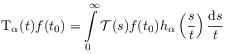 |
(5) |
where ![]() and
and ![]() .
[90.1.2] Explicit expressions for the kernels
.
[90.1.2] Explicit expressions for the kernels ![]() for all
for all ![]() are given in eq. (69) below.
[90.1.3] It is the main objective of this chapter to
show that (in a certain sense) all macroscopic
time evolutions have the form of eq. (5),
and that fractional time derivatives
are their infinitesimal generators.
are given in eq. (69) below.
[90.1.3] It is the main objective of this chapter to
show that (in a certain sense) all macroscopic
time evolutions have the form of eq. (5),
and that fractional time derivatives
are their infinitesimal generators.
[90.2.1] Given the great difference between ![]() in
eq. (5)
and
in
eq. (5)
and ![]() in eq. (4) it
becomes clear that basic issues, such as irreversibility,
translation symmetry, or the meaning of stationarity
are inevitably involved when proposing fractional dynamics.
[90.2.2] Let me therefore advance the basic postulate that all time
evolutions of physical systems are irreversible.
[90.2.3] Obviously this law of irreversibility must
be considered to be an empirical law of nature
equal in rank to the law of energy conservation.
[90.2.4] Reversible behaviour is an idealization.
[90.2.5] Its validity or applicability in physical experiments
depends on the degree to which the system can be isolated
(or decoupled) from its past history and its environment.
[90.2.6] According to this view the irreversible flow of time
is more fundamental than the time reversal symmetry of Newtons
or other equations.
[90.2.7] My starting point is therefore that for a general time
evolution operator
in eq. (4) it
becomes clear that basic issues, such as irreversibility,
translation symmetry, or the meaning of stationarity
are inevitably involved when proposing fractional dynamics.
[90.2.2] Let me therefore advance the basic postulate that all time
evolutions of physical systems are irreversible.
[90.2.3] Obviously this law of irreversibility must
be considered to be an empirical law of nature
equal in rank to the law of energy conservation.
[90.2.4] Reversible behaviour is an idealization.
[90.2.5] Its validity or applicability in physical experiments
depends on the degree to which the system can be isolated
(or decoupled) from its past history and its environment.
[90.2.6] According to this view the irreversible flow of time
is more fundamental than the time reversal symmetry of Newtons
or other equations.
[90.2.7] My starting point is therefore that for a general time
evolution operator ![]() the evolution parameter
the evolution parameter ![]() is not a time instant (which could be positive
or negative), but a duration, which cannot be negative.
is not a time instant (which could be positive
or negative), but a duration, which cannot be negative.
[90.3.1] An immediate consequence of the postulated law of irreversibility is that the classical irreversibility problem of theoretical physics becomes reversed.
[page 91, §0]
[91.0.1] Now the theoretical task is not to explain how irreversibility
arises from reversible evolution equations, but how seemingly
reversible equations arise as idealizations from
an underlying irreversible time evolution.
[91.0.2] A possible explanation is provided by the present
theory based on eq. (5).
[91.0.3] It turns out that the case ![]() in eq. (5)
is of predominant mathematical and physical importance, because it
is in a quantifiable sense a strong universal attractor.
[91.0.4] In this case the kernel
in eq. (5)
is of predominant mathematical and physical importance, because it
is in a quantifiable sense a strong universal attractor.
[91.0.4] In this case the kernel ![]() becomes
becomes
| (6) |
and the time evolution ![]() in (5)
reduces to a simple translation as in eq.(4).
[91.0.5]
in (5)
reduces to a simple translation as in eq.(4).
[91.0.5] ![]() with
with ![]() is a
representation of the time semigroup (
is a
representation of the time semigroup (![]() ).
[91.0.6] It can be extended to one of the full group (
).
[91.0.6] It can be extended to one of the full group (![]() ).
[91.0.7] This is not possible for
).
[91.0.7] This is not possible for ![]() with
with ![]() .
[91.0.8] The physical interpretation of
.
[91.0.8] The physical interpretation of ![]() is seen from
is seen from
![]() for
for ![]() and
and ![]() for
for ![]() .
[91.0.9] Hence the parameter
.
[91.0.9] Hence the parameter ![]() classifies and quantifies
the influence of the past history.
[91.0.10] Small values of
classifies and quantifies
the influence of the past history.
[91.0.10] Small values of ![]() correspond to a strong influence of
the past history.
[91.0.11] For
correspond to a strong influence of
the past history.
[91.0.11] For ![]() the influence of
the past history is minimal in the sense that
it enters only through the present state.
the influence of
the past history is minimal in the sense that
it enters only through the present state.
[91.1.1] The basic result in eq. (5) was
given in [6] and subsequently rationalized
within ergodic theory by investigating the
recurrence properties of induced automorphisms
on subsets of measure zero [9, 10, 11].
[91.1.2] In these investigations the existence of a recurrent
subset of measure zero had to be assumed.
[91.1.3] Such an assumption becomes plausible from observations
in low dimensional chaotic systems
(see e.g. [25, 26] and Chapter V).
[91.1.4] A rigorous proof for any given dynamical
system, however, appears difficult, and it is therefore
of interest to rederive the emergence of ![]() from a different, and more general, approach.
from a different, and more general, approach.
