2 Foundations

2.1 Basic Desiderata for Time Evolutions

[91.2.1] The following basic requirements define a time evolution in this chapter.

Semigroup
[91.2.2] A time evolution is a pair $(\{\mbox{\rm T}_{\tau}(t):0\leq t<\infty\},(B_{\tau},\|\cdot\|))$ where $\mbox{\rm T}_{\tau}(t)=\mbox{\rm T}(t\tau)$ is a semigroup of operators $\{\mbox{\rm T}(t):0\leq t<\infty\}$ mapping the Banach space $(B_{\tau}(\mathbb{R}),\|\cdot\|)$ of functions $f_{\tau}(s)=f(s\tau)$ on $\mathbb{R}$ to itself. [91.2.3] The argument $t\geq 0$ of $\mbox{\rm T}_{\tau}(t)$ represents a time duration, the argument $s\in\mathbb{R}$ of $f_{\tau}(s)$ a time instant. [91.2.4] The index $\tau>0$ indicates the units (or scale) of time. [91.2.5] Below, $\tau$ will again be frequently suppressed to simplify the notation. [91.2.6] The elements $f_{\tau}(s)=f(s\tau)\in B_{\tau}$ represent observables or

[page 92, §0]

the state of a physical system as function of the time coordinate $s\in\mathbb{R}$ . [92.0.1] The semigroup conditions require

$\displaystyle\mbox{\rm T}_{\tau}(t_{1})\mbox{\rm T}_{\tau}(t_{2})f_{\tau}(t_{0})$ $\displaystyle=\mbox{\rm T}_{\tau}(t_{1}+t_{2})f_{\tau}(t_{0})$ (7)

$\displaystyle\mbox{\rm T}_{\tau}(0)f_{\tau}(t_{0})$ $\displaystyle=f_{\tau}(t_{0})$ (8)

for $t_{1},t_{2}>0$ , $t_{0}\in\mathbb{R}$ and $f_{\tau}\in B_{\tau}$ . [92.0.2] The first condition may be viewed as representing the unlimited divisibility of time.
Continuity
[92.0.3] The time evolution is assumed to be strongly continuous in $t$ by demanding

$\lim _{{t\to 0}}\|\mbox{\rm T}(t)f-f\|=0$ (9)

for all $f\in B$ .
Homogeneity
[92.0.4] The homogeneity of the time coordinate requires commutativity with translations

${\mathcal{T}}({t_{1}})\mbox{\rm T}(t_{2})f(t_{0})=\mbox{\rm T}(t_{2}){\mathcal{T}}({t_{1}})f(t_{0})$ (10)

for all $t_{2}>0$ and $t_{0},t_{1}\in\mathbb{R}$ . [92.0.5] This postulate allows to shift the origin of time and it reflects the basic symmetry of time translation invariance.
Causality
[92.0.6] The time evolution operator should be causal in the sense that the function $g(t_{0})=(\mbox{\rm T}(t)f)(t_{0})$ should depend only on values of $f(s)$ for $s<t_{0}$ .
Coarse Graining
[92.0.7] A time evolution operator $\mbox{\rm T}(t)$ should be obtainable from a coarse graining procedure. [92.0.8] A precise definition of coarse graining is given in Definition 2.3 below. [92.0.9] The idea is to combine a time average $\frac{1}{t}\int _{{s-t}}^{s}f(t^{{\prime}})\;\mbox{\rm d}t^{{\prime}}$ in the limit $t,s\to\infty$ with a rescaling of $s$ and $t$ .

[92.0.10] While the first four requirements are conventional the fifth requires comment. [92.0.11] Averages over long intervals may themselves be timedependent on much longer time scales. [92.0.12] An example would be the position of an atom in a glass. [92.0.13] On short time scales the position fluctuates rapidly around a well defined average position. [92.0.14] On long time scales the structural relaxation processes in the glass can change this average position. [92.0.15] The purpose of any coarse graining procedure is to connect microscopic to macroscopic scales. [92.0.16] Of course, what is microscopic

[page 93, §0] depends on the physical situation. [93.0.1] Any microscopic time evolution may itself be viewed as macroscopic from the perspective of an underlying more microscopic theory. [93.0.2] Therefore it seems physically necessary and natural to demand that a time evolution should generally be obtainable from a coarse graining procedure.

2.2 Evolutions, Convolutions and Averages

[93.1.1] There is a close connection and mathematical similarity between the simplest time evolution $\mbox{\rm T}(t)={\mathcal{T}}(t)$ and the operator $\mbox{\rm M}(t)$ of time averaging defined as the mathematical mean

$\mbox{\rm M}(t)f(s)=\frac{1}{t}\int^{s}_{{s-t}}f(y)\;\mbox{\rm d}y,$

(11)

where $t>0$ is the length of the averaging interval. [93.1.2] Rewriting this formally as

$\mbox{\rm M}(t)f(s)=\frac{1}{t}\int^{t}_{0}f(s-y)\;\mbox{\rm d}y=\frac{1}{t}\int^{t}_{0}{\mathcal{T}}(y)f(s)\;\mbox{\rm d}y$

(12)

exhibits the relation between $\mbox{\rm M}(t)$ and ${\mathcal{T}}(t)$ . [93.1.3] It shows also that $\mbox{\rm M}(t)$ commutes with translations (see eq. (10)).

[93.2.1] A second even more suggestive relationship between $\mbox{\rm M}(t)$ and ${\mathcal{T}}(t)$ arises because both operators can be written as convolutions. [93.2.2] The operator $\mbox{\rm M}(t)$ may be written as

$\mbox{\rm M}(t)f(s)=\frac{1}{t}\int^{t}_{0}f(s-y)\;\mbox{\rm d}y=\int^{\infty}_{{-\infty}}f(s-y)\frac{1}{t}\chi _{{[0,1]}}\left(\frac{y}{t}\right)\;\mbox{\rm d}y=\int^{s}_{0}f(s-y)\frac{1}{t}\chi _{{[0,1]}}\left(\frac{y}{t}\right)\;\mbox{\rm d}y,$

(13)

where the kernel

$\chi _{{[0,1]}}(x)=\begin{cases}1&\text{\ \ \ \ for }x\in[0,1]\\ 0&\text{\ \ \ \ for }x\notin[0,1]\end{cases}$

(14)

is the characteristic function of the unit interval. [93.2.3] The Laplace convolution in the last line requires $t<s$ . [93.2.4] The translations ${\mathcal{T}}(t)$ on the other hand may be

[page 94, §0] written as

${\mathcal{T}}(t)f(s)=f(s-t)=\int _{{-\infty}}^{{\infty}}f(s-y)\frac{1}{t}\delta\left(\frac{y}{t}-1\right)\;\mbox{\rm d}y=\int _{{0}}^{{s}}f(s-y)\frac{1}{t}\delta\left(\frac{y}{t}-1\right)\;\mbox{\rm d}y$

(15)

where again $0<t<s$ is required for the Laplace convolution in the last equation. [94.0.1] The similarity between eqs. (15) and (13) suggests to view the time translations ${\mathcal{T}}(t)$ as a degenerate form of averaging $f$ over a single point. [94.0.2] The operators $\mbox{\rm M}(t)$ and ${\mathcal{T}}(t)$ are both convolution operators. [94.0.3] By Lebesgues theorem $\lim _{{t\to 0}}\mbox{\rm M}(t)f(s)=f(s)$ so that $\mbox{\rm M}(0)f(t)=f(t)$ in analogy with eq. (8) which holds for ${\mathcal{T}}(t)$ . [94.0.4] However, while the translations ${\mathcal{T}}(t)$ fulfill eq. (7) and form a convolution semigroup whose kernel is the Dirac measure at 1, the averaging operators $\mbox{\rm M}(t)$ do not form a semigroup as will be seen below.

[94.1.1] The appearance of convolutions and convolution semigroups is not accidental. [94.1.2] Convolution operators arise quite generally from the symmetry requirement of eq. (10) above. [94.1.3] Let $L^{p}(\mathbb{R}^{n})$ denote the Lebesgue spaces of $p$ -th power integrable functions, and let ${\mathcal{S}}$ denote the Schwartz space of test functions for tempered distributions [27]. [94.1.4] It is well established that all bounded linear operators on $L^{p}(\mathbb{R}^{n})$ commuting with translations (i.e. fulfilling eq. (10)) are of convolution type [27].

Theorem 2.1

[94.1.5] Suppose the operator $\mbox{\rm B}:L^{p}(\mathbb{R}^{n})\to L^{q}(\mathbb{R}^{n})$ , $1\leq p,q,\leq\infty$ is linear, bounded and commutes with translations. [94.1.6] Then there exists a unique tempered distribution $g$ such that $\mbox{\rm B}h=g*h$ for all $h\in{\mathcal{S}}$ .

[94.2.1] For $p=q=1$ the tempered distributions in this theorem are finite Borel measures. [94.2.2] If the measure is bounded and positive this means that the operator B can be viewed as a weighted averaging operator. [94.2.3] In the following the case $n=1$ will be of interest. [94.2.4] A positive bounded measure $\mu$ on $\mathbb{R}$ is uniquely determined by its distribution function $\widetilde{\mu}:\mathbb{R}\to[0,1]$ defined by

$\widetilde{\mu}(x)=\frac{\mu(]-\infty,x[)}{\mu(\mathbb{R})}.$

(16)

[94.2.5] The tilde will again be omitted to simplify the notation. [94.2.6] Physically a weighted average $\mbox{\rm M}(t;\mu)f(s)$ represents the measurement of a signal $f(s)$ using an apparatus with response characterized by $\mu$ and resolution $t>0$ . [94.2.7] Note that the resolution (length of averaging interval) is a duration and cannot be negative.

[page 95, §1]

Definition 2.1 (Averaging)

[95.1.1] Let $\mu$ be a (probability) distribution function on $\mathbb{R}$ , and $t>0$ . [95.1.2] The weighted (time) average of a function $f$ on $\mathbb{R}$ is defined as the convolution

$\mbox{\rm M}(t;\mu)f(s)=(f*\mu(\cdot/t))(s)=\int _{{-\infty}}^{\infty}f(s-s^{{\prime}})\;\mbox{\rm d}\mu(s^{{\prime}}/t)=\int _{{-\infty}}^{\infty}{\mathcal{T}}({s^{{\prime}}})f(s)\;\mbox{\rm d}\mu(s^{{\prime}}/t)$

(17)

whenever it exists. [95.1.3] The average is called causal if the support of $\mu$ is in $\mathbb{R}_{+}$ . [95.1.4] It is called degenerate if the support of $\mu$ consists of a single point.

[95.2.1] The weight function or kernel $m(x)$ corresponding to a distribution $\mu(x)$ is defined as $m(x)=\mbox{\rm d}\mu/\mbox{\rm d}x$ whenever it exists.

[95.3.1] The averaging operator $\mbox{\rm M}(t)$ in eq. (11) corresponds to a measure with distribution function

$\mu _{\chi}(x)=\begin{cases}0&\text{\ \ \ \ for }x\leq 0\\ x&\text{\ \ \ \ for }0\leq x\leq 1\\ 1&\text{\ \ \ \ for }x\geq 1\end{cases}$

(18)

while the time translation ${\mathcal{T}}(t)$ corresponds to the (Dirac) measure $\delta(x-1)$ concentrated at $1$ with distribution function

$\mu _{\delta}(x)=\begin{cases}0&\text{\ \ \ \ for }x<1\\ 1&\text{\ \ \ \ for }x\geq 1.\end{cases}$

(19)

[95.3.2] Both averages are causal, and the latter is degenerate.

[95.4.1] Repeated averaging leads to convolutions. [95.4.2] The convolution $\kappa$ of two distributions $\mu,\nu$ on $\mathbb{R}$ is defined through

$\kappa(x)=(\mu*\nu)(x)=\int _{{-\infty}}^{\infty}\mu(x-y)\mbox{\rm d}\nu(y)=\int _{{-\infty}}^{\infty}\nu(x-y)\mbox{\rm d}\mu(y).$

(20)

[95.4.3] The Fourier transform of a distribution is defined by

${\mathcal{F}}\left\{\mu(t)\right\}(\omega)=\widehat{\mu}(\omega)=\int _{{-\infty}}^{\infty}e^{{i\omega t}}\mbox{\rm d}\mu(t)=\int _{{-\infty}}^{\infty}e^{{i\omega t}}m(t)\;\mbox{\rm d}t$

(21)

where the last equation holds when the distribution admits a weight function. [95.4.4] A sequence $\mu _{n}(x)$ of distributions is said to converge weakly to a limit $\mu(x)$ ,

[page 96, §0] written as

$\lim _{{n\to\infty}}\mu _{n}=\mu,$

(22)

$\lim _{{n\to\infty}}\int _{{-\infty}}^{\infty}f(x)\mbox{\rm d}\mu _{n}(x)=\int _{{-\infty}}^{\infty}f(x)\mbox{\rm d}\mu _{(}x)$

(23)

holds for all bounded continuous functions $f$ .

[96.1.1] The operators $\mbox{\rm M}(t)$ and ${\mathcal{T}}(t)$ above have positive kernels, and preserve positivity in the sense that $f\geq 0$ implies $\mbox{\rm M}(t)f\geq 0$ . [96.1.2] For such operators one has

Theorem 2.2

[96.1.3] Let T be a bounded operator on $L^{p}(\mathbb{R})$ , $1\leq p<\infty$ that is translation invariant in the sense that

$\displaystyle\mbox{\rm T}{\mathcal{T}}(t)f={\mathcal{T}}(t)\mbox{\rm T}f$

(24)

for all $t\in\mathbb{R}$ and $f\in L^{p}(\mathbb{R})$ , and such that $f\in L^{p}(\mathbb{R})$ and $0\leq f\leq 1$ almost everywhere implies $0\leq\mbox{\rm T}f\leq 1$ almost everywhere. [96.1.4] Then there exists a uniquely determined bounded measure $\mu$ on $\mathbb{R}$ with mass $\mu(\mathbb{R})\leq 1$ such that

$\mbox{\rm T}f(t)=(\mu*f)(t)=\int _{{-\infty}}^{\infty}f(t-s)\mbox{\rm d}\mu(s)$

(25)

Proof.

[96.1.5] For the proof see [28]. ∎

[96.1.6] The preceding theorem suggests to represent those time evolutions that fulfill the requirements 1.– 4. of the last section in terms of convolution semigroups of measures.

Definition 2.2 (Convolution semigroup)

[96.1.7] A family $\{\mu _{t}:t>0\}$ of positive bounded measures on $\mathbb{R}$ with the properties that

$\displaystyle\mu _{t}(\mathbb{R})$	$\displaystyle\leq 1\text{\ \ \ \ }{\rm for~}t>0,$	(26)
$\displaystyle\mu _{{t+s}}$	$\displaystyle=\mu _{t}*\mu _{s}\text{\ \ \ \ }{\rm for~}t,s>0,$	(27)
$\displaystyle\delta$	$\displaystyle=\lim _{{t\to 0}}\mu _{t}\text{\ \ \ \ }$	(28)

is called a convolution semigroup of measures on $\mathbb{R}$ .

[page 97, §1] [97.1.1] Here $\delta$ is the Dirac measure at $0$ and the limit is the weak limit. [97.1.2] The desired characterization of time evolutions now becomes

Corollary 2.1

[97.1.3] Let $\mbox{\rm T}(t)$ be a strongly continuous time evolution fulfilling the conditions of homogeneity and causality, and being such that $f\in L^{p}(\mathbb{R})$ and $0\leq f\leq 1$ almost everywhere implies $0\leq\mbox{\rm T}f\leq 1$ almost everywhere. [97.1.4] Then $\mbox{\rm T}(t)$ corresponds uniquely to a convolution semigroup of measures $\mu _{t}$ through

$\mbox{\rm T}(t)f(s)=(\mu _{t}*f)(s)=\int _{{-\infty}}^{\infty}f(s-s^{{\prime}})\mbox{\rm d}\mu _{t}(s^{{\prime}})$

(29)

with $\mathrm{supp}\,\mu _{t}\subset\mathbb{R}_{+}$ for all $t\geq 0$ .

Proof.

[97.1.5] Follows from Theorem 2.2 and the observation that $\mathrm{supp}\,\mu _{t}\cap\mathbb{R}_{-}\neq\emptyset$ would violate the causality condition. ∎

[97.2.1] Equation (29) establishes the basic convolution structure of the assertion in eq. (5). [97.2.2] It remains to investigate the requirement that $\mbox{\rm T}(t)$ should arise from a coarse graining procedure, and to establish the nature of the kernel in eq. (5).

2.3 Time Averaging and Coarse Graining

[97.3.1] The purpose of this section is to motivate the definition of coarse graining. [97.3.2] A first possible candidate for a coarse grained macroscopic time evolution could be obtained by simply rescaling the time in a microscopic time evolution as

$\mbox{\rm T}_{\infty}({\overline{t}})f(s)=\lim _{{\tau\to\infty}}\mbox{\rm T}_{\tau}({\overline{t}})f(s)=\lim _{{\tau\to\infty}}\mbox{\rm T}(\tau{\overline{t}})f(s)=\lim _{{\tau\to\infty}}f(s-\tau{\overline{t}})$

(30)

where $0<{\overline{t}}<\infty$ would be macroscopic times. [97.3.3] However, apart from special cases, the limit will in general not exist. [97.3.4] Consider for example a sinusoidal $f(t)$ oscillating around a constant. [97.3.5] Also, the infinite translation $\mbox{\rm T}_{\infty}$ is not an average, and this conflicts with the requirement above, that coarse graining should be a smoothing operation.

[97.4.1] A second highly popular candidate for coarse graining is therefore the averaging operator $\mbox{\rm M}(t)$ . [97.4.2] If the limit $t\to\infty$ exists and $f(t)$ is integrable in the finite interval $[s_{1},s_{2}]$ then the average

${\overline{f}}=\lim _{{t\to\infty}}\mbox{\rm M}(t)f(s_{1})=\lim _{{t\to\infty}}\mbox{\rm M}(t)f(s_{2})$

(31)

is a number independent of the instant $s_{i}$ . [97.4.3] Thus, if one wants to study the macroscopic time dependence of ${\overline{f}}$ , it is necessary to consider a scaling limit in

[page 98, §0] which also $s\to\infty$ . [98.0.1] If the scaling limit $s,t\to\infty$ is performed such that $s/t={\overline{s}}$ is constant, then

$\lim _{{\substack{t,s\to\infty\\ s=t{\overline{s}}}}}\mbox{\rm M}(t)f(s)=\int _{{{\overline{s}}-1}}^{{{\overline{s}}}}f_{\infty}(z)\;\mbox{\rm d}z=\mbox{\rm M}(1)f_{\infty}({\overline{s}})$

(32)

becomes again an averaging operator over the infinitely rescaled observable. [98.0.2] Now $\mbox{\rm M}(1)$ still does not qualify as a coarse grained time evolution because $\mbox{\rm M}(1)\mbox{\rm M}(1)\neq\mbox{\rm M}(2)$ as will be shown next.

[98.1.1] Consider again the operator $\mbox{\rm M}(t)$ defined in eq. (11). [98.1.2] It follows that

$\mbox{\rm M}^{2}(t)f(s)=\left(\frac{1}{t}\chi _{{[0,1]}}\left(\frac{\cdot}{t}\right)*\frac{1}{t}\chi _{{[0,1]}}\left(\frac{\cdot}{t}\right)*f\right)(s)$

(33)

and

$\frac{1}{t^{2}}\int^{x}_{0}\chi _{{[0,1]}}\left(\frac{x-y}{t}\right)\chi _{{[0,1]}}\left(\frac{y}{t}\right)\;\mbox{\rm d}y=\begin{cases}0&\text{\ \ \ \ for }x\leq 0\\ \frac{x}{t^{2}}&\text{\ \ \ \ for }0\leq x\leq t\\ \frac{2}{t}-\frac{x}{t^{2}}&\text{\ \ \ \ for }t\leq x\leq 2t\\ 0&\text{\ \ \ \ for }x\geq 2t.\end{cases}$

(34)

[98.1.3] Thus twofold averaging may be written as

$\mbox{\rm M}^{2}(t)f(s)=\int _{0}^{s}f(s-y)\frac{1}{t}\chi^{{(2)}}\left(\frac{y}{t}\right)\;\mbox{\rm d}y$

(35)

where

$\chi^{{(2)}}(x)=\begin{cases}x&\text{\ \ \ \ for $0\leq x\leq 1$}\\ 2-x&\text{\ \ \ \ for $1\leq x\leq 2$}\\ 0&\text{\ \ \ \ otherwise}\end{cases}$

(36)

is the new kernel. [98.1.4] It follows that $\mbox{\rm M}^{2}(t)\neq\mbox{\rm M}(2t)$ , and hence the averaging operators $\mbox{\rm M}(t)$ do not form a semigroup.

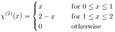
[98.2.1] Although $\mbox{\rm M}^{2}(t)\neq\mbox{\rm M}(2t)$ the iterated average is again a convolution operator with support $[0,2t]$ compared to $[0,t]$ for $\mbox{\rm M}(t)$ . [98.2.2] Similarly, $\mbox{\rm M}^{3}(t)$ has support $[0,3t]$ . [98.2.3] This suggests to investigate the iterated average $\mbox{\rm M}^{n}(t)f(s)$ in a scaling limit $n,s\to\infty$ . [98.2.4] The limit $n\to\infty$ smoothes the function by enlarging the

[page 99, §0] averaging window to $[0,nt]$ , and the limit $s\to\infty$ shifts the origin to infinity. [99.0.1] The result may be viewed as a coarse grained time evolution in the sense of a time evolution on time scales "longer than infinitely long". [99.0.2] ^c (This is a footnote:) ^c The scaling limit was called "ultralong time limit" in [10] It is therefore necessary to rescale $s$ . [99.0.3] If the rescaling factor is called $\sigma _{n}>0$ one is interested in the limit $n,s\to\infty$ with ${\overline{s}}=s/\sigma _{n}$ fixed, and $\sigma _{n}\to\infty$ with $n\to\infty$ and fixed $t>0$

$\lim _{{\substack{n,s\to\infty\\ s=\sigma _{n}{\overline{s}}}}}(\mbox{\rm M}(t)^{n}f)(s)=\lim _{{n\to\infty}}(\mbox{\rm M}(t)^{n}f)(\sigma _{n}{\overline{s}})$

(37)

whenever this limit exists. [99.0.4] Here ${\overline{s}}>1$ denotes the macroscopic time.

[99.1.1] To evaluate the limit note first that eq. (11) implies

$\mbox{\rm M}(t)f(\sigma _{n}{\overline{s}})=\int^{{{\overline{s}}}}_{0}f_{{\sigma _{n}}}({\overline{s}}-z)\frac{\sigma _{n}}{t}\chi _{{[0,1]}}\left(\frac{\sigma _{n}z}{t}\right)\;\mbox{\rm d}z$

(38)

where $f_{\tau}(t)=f(t\tau)$ denotes the rescaled observable with a rescaling factor $\tau$ . [99.1.2] The $n$ -th iterated average may now be calculated by Laplace transformation with respect to ${\overline{s}}$ . [99.1.3] Note that

${\mathcal{L}}\left\{\frac{1}{c}\chi _{{[0,1]}}\left(\frac{x}{c}\right)\right\}(u)=\frac{1-e^{{-cu}}}{cu}=E_{{1,2}}(-cu)$

(39)

for all $c\in\mathbb{R}$ , where $E_{{1,2}}(x)$ is the generalized Mittag-Leffler function defined as

$E_{{a,b}}(x)=\sum _{{k=0}}^{\infty}\frac{x^{k}}{\Gamma(ak+b)}$

(40)

for all $a>0$ and $b\in\mathbb{C}$ . [99.1.4] Using the general relation

$E_{{a,b}}(x)=\frac{1}{\Gamma(b)}+xE_{{a,a+b}}(x)$

(41)

gives with eqs. (37) and (38)

${\mathcal{L}}\left\{\mbox{\rm M}(t)^{n}f(\sigma _{n}{\overline{s}})\right\}({\overline{u}})=\left(1-\frac{t{\overline{u}}}{\sigma _{n}}E_{{1,3}}\left(-\frac{t{\overline{u}}}{\sigma _{n}}\right)\right)^{n}\frac{1}{\sigma _{n}}{\mathcal{L}}\left\{ f(s)\right\}\left(\frac{{\overline{u}}}{\sigma _{n}}\right)$

(42)

where $f({\overline{u}})$ is the Laplace transform of $f({\overline{s}})$ . [99.1.5] Noting that $E_{{1,3}}(0)=1/2$ it becomes apparent that a limit $n\to\infty$ will exist if the rescaling factors are

[page 100, §0] chosen as $\sigma _{n}\sim n$ . [100.0.1] With the choice $\sigma _{n}=\sigma n/2$ and $\sigma>0$ one finds for the first factor

$\lim _{{n\to\infty}}\left(1-\frac{2t{\overline{u}}}{n\sigma}E_{{1,3}}\left(-\frac{2t{\overline{u}}}{n\sigma}\right)\right)^{n}=e^{{-t{\overline{u}}/\sigma}}.$

(43)

[100.0.2] Concerning the second factor assume that for each ${\overline{u}}$ the limit

$\lim _{{n\to\infty}}\frac{2}{n}{\mathcal{L}}\left\{ f(s)\right\}\left(\frac{2{\overline{u}}}{n}\right)={\overline{f}}({\overline{u}})$

(44)

exists and defines a function ${\overline{f}}({\overline{u}})$ . [100.0.3] Then

$\lim _{{n\to\infty}}\frac{1}{\sigma _{n}}{\mathcal{L}}\left\{ f({\overline{s}})\right\}\left(\frac{{\overline{u}}}{\sigma _{n}}\right)=\frac{1}{\sigma}{\overline{f}}\left(\frac{{\overline{u}}}{\sigma}\right),$

(45)

and it follows that

$\lim _{{n\to\infty}}{\mathcal{L}}\left\{\mbox{\rm M}(t)^{n}f(\sigma _{n}{\overline{s}})\right\}({\overline{u}})=e^{{-t{\overline{u}}/\sigma}}\frac{1}{\sigma}{\overline{f}}\left(\frac{{\overline{u}}}{\sigma}\right).$

(46)

[100.0.4] With ${\overline{t}}=t/\sigma$ Laplace inversion yields

$\lim _{{\substack{n,s\to\infty\\ s=\sigma _{n}{\overline{s}}}}}(\mbox{\rm M}(t)^{n}f)(s)=\int _{{0}}^{{{\overline{s}}}}{\overline{f}}(\sigma{\overline{s}}-\sigma{\overline{y}})\delta({\overline{y}}-{\overline{t}})\;\mbox{\rm d}{\overline{y}}={\overline{f}}_{\sigma}({\overline{s}}-{\overline{t}}).$

(47)

[100.0.5] Using eq. (12) the result (47) may be expressed symbolically as

$\lim _{{\substack{n,s\to\infty\\ s/n=\sigma{\overline{s}}/2}}}\left(\frac{1}{t}\int^{t}_{0}{\mathcal{T}}(y)\;\mbox{\rm d}y\right)^{n}f(s)={\overline{f}}_{\sigma}({\overline{s}}-{\overline{t}})=\overline{{\mathcal{T}}}({{\overline{t}}})\;{\overline{f}}_{\sigma}({\overline{s}})$

(48)

with ${\overline{t}}=t/\sigma$ . [100.0.6] This expresses the macroscopic or coarse grained time evolution $\overline{{\mathcal{T}}}({{\overline{t}}})$ as the scaling limit of a microscopic time evolution ${\mathcal{T}}(t)$ . [100.0.7] Note that there is some freedom in the choice of the rescaling factors $\sigma _{n}$ expressed by the prefactor $\sigma$ . [100.0.8] This freedom reflects the freedom to choose the time units for the coarse grained time evolution.

[100.1.1] The coarse grained time evolution $\overline{{\mathcal{T}}}({{\overline{t}}})$ is again a translation. [100.1.2] The coarse grained observable ${\overline{f}}({\overline{s}})$ corresponds to a microscopic average by virtue of the following result [29].

[page 101, §1]

Proposition 2.1

[101.1.1] If $f(x)$ is bounded from below and one of the limits

$\lim _{{y\to\infty}}\frac{1}{y}\int _{0}^{y}f(x)\;\mbox{\rm d}x$

$\lim _{{z\to 0}}z\int _{0}^{\infty}f(x)e^{{-zx}}\;\mbox{\rm d}x$

exists then the other limit exists and

$\lim _{{y\to\infty}}\frac{1}{y}\int _{0}^{y}f(x)\;\mbox{\rm d}x=\lim _{{z\to 0}}z{\mathcal{L}}\left\{ f(x)\right\}(z).$

(49)

[101.1.2] Comparison of the last relation with eq. (44) shows that ${\overline{f}}({\overline{s}})$ is a microscopic average of $f(s)$ . [101.1.3] While $s$ is a microscopic time coordinate, the time coordinate ${\overline{s}}$ of ${\overline{f}}$ is macroscopic.

[101.2.1] The preceding considerations justify to view the time evolution $\overline{{\mathcal{T}}}({{\overline{t}}})$ as a coarse grained time evolution. [101.2.2] Every observation or measurement of a physical quantity $f(s)$ requires a minimum duration $t$ determined by the temporal resolution of the measurement apparatus. [101.2.3] The value $f(s)$ at the time instant $s$ is always an average over this minimum time interval. [101.2.4] The averaging operator $\mbox{\rm M}(t)$ with kernel $\chi _{{[0,1]}}$ defined in equation (11) represents an idealized averaging apparatus that can be switched on and off instantaneously, and does not otherwise influence the measurement. [101.2.5] In practice one is usually confronted with finite startup and shutdown times and a nonideal response of the apparatus. [101.2.6] These imperfections are taken into account by using a weighted average with a weight function or kernel that differs from $\chi _{{[0,1]}}$ . [101.2.7] The weight function reflects conditions of the measurement, as well as properties of the apparatus and its interaction with the system. [101.2.8] It is therefore of interest to consider causal averaging operators $\mbox{\rm M}(t;\mu)$ defined in eq. (17) with general weight functions. [101.2.9] A general coarse graining procedure is then obtained from iterating these weighted averages.

Definition 2.3 (Coarse Graining)

[101.2.10] Let $\mu$ be a probability distribution on $\mathbb{R}$ , and $\sigma _{n}>0$ , $n\in\mathbb{N}$ a sequence of rescaling factors. A coarse graining limit is defined as

$\lim _{{\substack{n,s\to\infty\\ s=\sigma _{n}{\overline{s}}}}}(\mbox{\rm M}(t;\mu)^{n}f)(s)$

(50)

[page 102, §0] whenever the limit exists. [102.0.1] The coarse graining limit is called causal if $\mbox{\rm M}(t;\mu)$ is causal, i.e. if $\mathrm{supp}\,\mu\subset\mathbb{R}_{+}$ .

2.4 Coarse Graining Limits and Stable Averages

[102.1.1] The purpose of this section is to investigate the coarse graining procedure introduced in Definition 2.3. [102.1.2] Because the coarse graining procedure is defined as a limit it is useful to recall the following well known result for limits of distribution functions [30]. [102.1.3] For the convenience of the reader its proof is reproduced in the appendix.

Proposition 2.2

[102.1.4] Let $\mu _{n}(s)$ be a weakly convergent sequence of distribution functions. [102.1.5] If $\lim _{{n\to\infty}}\mu _{n}(s)=\mu(s)$ , where $\mu(s)$ is nondegenerate then for any choice of $a_{n}>0$ and $b_{n}$ there exist $a>0$ and $b$ such that

$\lim _{{n\to\infty}}\mu _{n}(a_{n}x+b_{n})=\mu(ax+b).$

(51)

[102.2.1] The basic result for coarse graining limits can now be formulated.

Theorem 2.3 (Coarse Graining Limit)

[102.2.2] Let $f(s)$ be such that the limit $\lim _{{a\to 0}}a\widehat{f}(a\omega)=\widehat{{\overline{f}}}(\omega)$ defines the Fourier transform of a function ${\overline{f}}(s)$ . [102.2.3] Then the coarse graining limit exists and defines a convolution operator

$\lim _{{\substack{n,s\to\infty\\ s=\sigma _{n}{\overline{s}}}}}(\mbox{\rm M}(t;\mu)^{n}f)(s)=\int _{{-\infty}}^{\infty}{\overline{f}}({\overline{s}}-{\overline{s}}^{{\prime}})\;\mbox{\rm d}\nu({\overline{s}}^{{\prime}}/t;\mu)$

(52)

if and only if for any $a_{1},a_{2}>0$ there are constants $a>0$ and $b$ such that the distribution function $\nu(x)=\nu(x;\mu)$ obeys the relation

$\nu(a_{1}x)*\nu(a_{2}x)=\nu(ax+b).$

(53)

Proof.

[102.2.4] In the previous section the coarse graining limit was evaluated for the distribution $\mu _{\chi}$ from eq. (18) and the corresponding $\nu$ was found in eq. (47) to be degenerate. [102.2.5] A degenerate distribution $\nu$ trivially obeys eq. (53). [102.2.6] Assume therefore from now on that neither $\mu$ nor $\nu$ are degenerate.

[102.3.1] Employing equation (17) in the form

$\mbox{\rm M}(t;\mu)f(\sigma _{n}{\overline{s}})=\int _{{-\infty}}^{\infty}f(\sigma _{n}{\overline{s}}-\sigma _{n}y)\mbox{\rm d}\mu(\sigma _{n}y/t)$

(54)

[page 103, §0] one computes the Fourier transformation of $\mbox{\rm M}(t;\mu)^{n}f$ with respect to ${\overline{s}}$

${\mathcal{F}}\left\{\mbox{\rm M}(t;\mu)^{n}f(\sigma _{n}{\overline{s}})\right\}({\overline{\omega}})=\left[\widehat{\mu}\left(\frac{t{\overline{\omega}}}{\sigma _{n}}\right)\right]^{n}\frac{1}{\sigma _{n}}\widehat{f}\left(\frac{{\overline{\omega}}}{\sigma _{n}}\right).$

(55)

[103.0.1] By assumption $\widehat{f}({\overline{\omega}}/\sigma _{n})/\sigma _{n}$ has a limit whenever $\sigma _{n}\to\infty$ with $n\to\infty$ . [103.0.2] Thus the coarse graining limit exists and is a convolution operator whenever $[\widehat{\mu}(t{\overline{\omega}}/\sigma _{n})]^{n}$ converges to $\widehat{\nu}({\overline{\omega}})$ as $n\to\infty$ . [103.0.3] Following [30] it will be shown that this is true if and only if the characterization (53) and $\sigma _{n}\to\infty$ with $n\to\infty$ apply. [103.0.4] To see that

$\lim _{{n\to\infty}}\sigma _{n}=\infty$

(56)

holds, assume the contrary. Then there is a subsequence $\sigma _{{n_{k}}}$ converging to a finite limit. [103.0.5] Thus

$|\widehat{\mu}(t\omega/\sigma _{{n_{k}}})|^{{n_{k}}}=|\widehat{\nu}(\omega)|(1+{\it o}(1))$

(57)

so that

$|\widehat{\mu}(\omega)|=|\widehat{\nu}(\omega\sigma _{{n_{k}}}/t)|^{{1/n_{k}}}(1+{\it o}(1))$

(58)

for all $\omega$ . [103.0.6] As $n_{k}\to\infty$ this leads to $|\widehat{\mu}(\omega)|=1$ for all $\omega$ and hence $\mu$ must be degenerate contrary to assumption.

[103.1.1] Next, it will be shown that

$\lim _{{n\to\infty}}\frac{\sigma _{{n+1}}}{\sigma _{n}}=1.$

(59)

[103.1.2] From eq. (56) it follows that $\lim _{{n\to\infty}}|\widehat{\mu}(\omega/\sigma _{n})|=1$ and therefore

$|\widehat{\mu}(t\omega/\sigma _{n})|^{n}=|\widehat{\nu}(\omega)|(1+{\it o}(1))$

(60)

and

$|\widehat{\mu}(t\omega/\sigma _{{n+1}})|^{{n+1}}=|\widehat{\nu}(\omega)|(1+{\it o}(1)).$

(61)

Substituting $\omega$ by $\sigma _{n}\omega/\sigma _{{n+1}}$ in eq. (60) and by $\sigma _{{n+1}}\omega/\sigma _{n}$ in eq. (61) shows that

$\lim _{{n\to\infty}}\left|\frac{\widehat{\nu}(\sigma _{{n+1}}\omega/\sigma _{n})}{\widehat{\nu}(\omega)}\right|=\lim _{{n\to\infty}}\left|\frac{\widehat{\nu}(\sigma _{n}\omega/\sigma _{{n+1}})}{\widehat{\nu}(\omega)}\right|=1.$

(62)

[page 104, §0] [104.0.1] If $\lim _{{n\to\infty}}\sigma _{{n+1}}/\sigma _{n}\neq 1$ then there exists a subsequence of either $(\sigma _{{n+1}}/\sigma _{n})$ or $(\sigma _{n}/\sigma _{{n+1}})$ converging to a constant $A<1$ . [104.0.2] Therefore eq. (62) implies $\widehat{\nu}(\omega)=\widehat{\nu}(A\omega)$ which upon iteration yields

$|\widehat{\nu}(\omega)|=|\widehat{\nu}(A^{n}\omega)|.$

(63)

[104.0.3] Taking the limit $n\to\infty$ then gives $|\widehat{\nu}(0)|=1$ implying that $\nu$ is degenerate contrary to assumption.

[104.1.1] Now let $0<a_{1}<a_{2}$ be two constants. [104.1.2] Because of (56) and (59) it is possible to choose for each $\varepsilon>0$ and sufficiently large $n>n_{0}(\varepsilon)$ an index $m(n)$ such that

$0\leq\frac{\sigma _{m}}{\sigma _{n}}-\frac{a_{2}}{a_{1}}<\varepsilon.$

(64)

[104.1.3] Consider the identity

$\left[\widehat{\mu}\left(\frac{a_{1}t{\overline{\omega}}}{\sigma _{n}}\right)\right]^{{n+m}}=\left[\widehat{\mu}\left(\frac{a_{1}t{\overline{\omega}}}{\sigma _{n}}\right)\right]^{n}\left[\widehat{\mu}\left(\frac{\sigma _{m}}{\sigma _{n}}\frac{a_{1}t{\overline{\omega}}}{\sigma _{m}}\right)\right]^{m}.$

(65)

By hypothesis the distribution functions corresponding to $\left[\widehat{\mu}\left(t{\overline{\omega}}/\sigma _{n}\right)\right]^{n}$ converge to $\nu({\overline{s}})$ as $n\to\infty$ . [104.1.4] Hence each factor on the right hand side converges and their product converges to $\nu(a_{1}{\overline{s}})*\nu(a_{2}{\overline{s}})$ . [104.1.5] It follows that the distribution function on the left hand side must also converge. [104.1.6] By Proposition 2.2 there must exist $a>0$ and $b$ such that the left hand side differs from $\nu({\overline{s}})$ only as $\nu(a{\overline{s}}+b)$ .

[104.2.1] Finally the converse direction that the coarse graining limit exists for $\mu=\nu$ is seen to follow from eq. (53). [104.2.2] This concludes the proof of the theorem. ∎

[104.3.1] The theorem shows that the coarse graining limit, if it exists, is again a macroscopic weighted average $\mbox{\rm M}(t;\nu)$ . [104.3.2] The condition (53) says that this macroscopic average has a kernel that is stable under convolutions, and this motivates the

Definition 2.4 (Stable Averages)

[104.3.3] A weighted averaging operator $\mbox{\rm M}(t;\mu)$ is called stable if for any $a_{1},a_{2}>0$ there are constants $a>0$ and $b\in\mathbb{R}$ such that

$\mu(a_{1}x)*\mu(a_{2}x)=\mu(ax+b)$

(66)

holds.

[104.4.1] This nomenclature emphasizes the close relation with the limit theorems of probability theory [30, 31]. [104.4.2] The next theorem provides the explicit form for distribution functions satisfying eq. (66). [104.4.3] The proof uses Bernsteins theorem and hence requires the concept of complete monotonicity.

[page 105, §1]

Definition 2.5

[105.1.1] A $C^{\infty}$ -function $f:]0,\infty[\to\mathbb{R}$ is called completely monotone if

$(-1)^{n}\frac{\mbox{\rm d}^{n}f}{\mbox{\rm d}x^{n}}\geq 0$

(67)

for all integers $n\geq 0$ .

[105.2.1] Bernsteins theorem [31, p. 439] states that a function is completely monotone if and only if it is the the Laplace transform ( $u>0$ )

$\mu(u)={\mathcal{L}}\left\{\mu(x)\right\}(u)=\int _{0}^{\infty}e^{{-ux}}\mbox{\rm d}\mu(x)=\int _{0}^{\infty}e^{{-ux}}m(x)\;\mbox{\rm d}x$

(68)

of a distribution $\mu$ or of a density $m=\mbox{\rm d}\mu/\mbox{\rm d}x$ .

[105.3.1] In the next theorem the explicit form of stable averaging kernels is found to be a special case of the general $H$ -function. [105.3.2] Because the $H$ -function will reappear in other results its general definition and properties are presented separately in Section 4.

Theorem 2.4

[105.3.3] A causal average is stable if and only if its weight function is of the form

$h_{\alpha}(x;b,c)=\frac{1}{b^{{1/\alpha}}}h_{\alpha}\left(\frac{x-c}{b^{{1/\alpha}}}\right)=\frac{1}{\alpha(x-c)}H_{{11}}^{{10}}\left(\frac{b^{{1/\alpha}}}{x-c}\left|\begin{array}[]{l}{(0,1)}\\ {(0,1/\alpha)}\end{array}\right.\right)$

(69)

where $0<\alpha\leq 1$ , $b>0$ and $c\in\mathbb{R}$ are constants and $h_{\alpha}(x)=h_{\alpha}(s;1,0)$ .

Proof.

[105.3.4] Let $c=0$ without loss of generality. [105.3.5] The condition (66) together with $\mathrm{supp}\,\mu\subset[0,\infty[$ defines one sided stable distribution functions [31]. [105.3.6] To derive the form (69) it suffices to consider condition (66) with $b=0$ . [105.3.7] Assume thence that for any $a_{1},a_{2}>0$ there exists $a>0$ such that

$\mu(a_{1}x)*\mu(a_{2}x)=\mu(ax)$

(70)

where the convolution is now a Laplace convolution because of the condition $\mathrm{supp}\,\subset[0,\infty[$ . [105.3.8] Laplace tranformation yields

$\mu(u/a_{1})\mu(u/a_{2})=\mu(u/a).$

(71)

[105.3.9] Iterating this equation (with $a_{1}=a_{2}=1$ ) shows that there is an $n$ -dependent constant $a(n)$ such that

$\mu(u)^{n}=\mu(u/a(n))$

(72)

[page 106, §0] and hence

$\mu\left(\frac{u}{a(nm)}\right)=\mu(u)^{{nm}}=\mu\left(\frac{u}{a(n)}\right)^{m}=\mu\left(\frac{u}{(a(n)a(m)}\right).$

(73)

[106.0.1] Thus $a(n)$ satisfies the functional equation

$a(nm)=a(n)a(m)$

(74)

whose solution is $a(n)=n^{{1/\gamma}}$ with some real constant written as $1/\gamma$ with hindsight. [106.0.2] Inserting $a(n)$ into eq.(72) and substituting the function $g(x)=\log\mu(x)$ gives

$ng(u)=g(un^{{-1/\gamma}}).$

(75)

[106.0.3] Taking logarithms and substituting $f(x)=\log g(e^{x})$ this becomes

$\log n+f(\log u)=f\left(\log u-\frac{\log n}{\gamma}\right).$

(76)

[106.0.4] The solution to this functional equation is $f(x)=-\gamma x$ . [106.0.5] Substituting back one finds $g(x)=x^{{-\gamma}}$ and therefore $\mu(u)$ is of the general form $\mu(u)=\exp(u^{{-\gamma}})$ with $\gamma\in\mathbb{R}$ . [106.0.6] Now $\mu$ is also a distribution function. Its normalization requires $\mu(u=0)=1$ and this restricts $\gamma$ to $\gamma<0$ . [106.0.7] Moreover, by Bernsteins theorem $\mu(u)$ must be completely monotone. [106.0.8] A completely monotone function is positive, decreasing and convex. [106.0.9] Therefore the power in the exponent must have a negative prefactor, and the exponent is restricted to the range $-1\leq\gamma<0$ . [106.0.10] Summarizing, the Laplace transform $\mu(u)$ of a distribution satisfying (70) is of the form

$\mu(u)=h_{\alpha}(u;b,0)=e^{{-bu^{\alpha}}}$

(77)

with $0<\alpha\leq 1$ and $b>0$ . [106.0.11] Checking that $h_{\alpha}(u;b,0)$ does indeed satisfy eq. (70) yields $a^{{-\alpha}}=a_{1}^{{-\alpha}}+a_{2}^{{-\alpha}}$ as the relation between the constants. [106.0.12] For the proof of the general case of eq. (66) see Refs. [30, 31].

[106.1.1] To invert the Laplace transform it is convenient to use the relation

${\mathcal{M}}\left\{ m(x)\right\}(s)=\frac{{\mathcal{M}}\left\{{\mathcal{L}}\left\{ m(x)\right\}(u)\right\}(1-s)}{\Gamma(1-s)}$

(78)

between the Laplace transform and the Mellin transform

${\mathcal{M}}\left\{ m(x)\right\}(s)=\int _{0}^{\infty}x^{{s-1}}m(t)\;\mbox{\rm d}x$

(79)

[page 107, §0] of a function $m(x)$ . [107.0.1] Using the Mellin transform [32]

${\mathcal{M}}\left\{ e^{{-bx^{\alpha}}}\right\}(s)=\frac{\Gamma(s/\alpha)}{\alpha b^{{s/\alpha}}}$

(80)

valid for $\alpha>0$ and $\mathrm{Re}\, s>0$ it follows that

${\mathcal{M}}\left\{ h_{\alpha}(x;b,0)\right\}(s)=\frac{1}{\alpha b^{{(1-s)/\alpha}}}\frac{\Gamma((1-s)/\alpha)}{\Gamma(1-s)}.$

(81)

[107.0.2] The general relation ${\mathcal{M}}\left\{ x^{{-1}}f(x^{{-1}})\right\}(s)={\mathcal{M}}\left\{ f(x)\right\}(1-s)$ then implies

${\mathcal{M}}\left\{ x^{{-1}}h_{\alpha}(x^{{-1}};b,0)\right\}(s)=\frac{1}{\alpha b^{{s/\alpha}}}\frac{\Gamma(s/\alpha)}{\Gamma(s)}$

(82)

which leads to

$x^{{-1}}h_{\alpha}(x^{{-1}};b,0)=\frac{1}{\alpha}H_{{11}}^{{10}}\left(b^{{1/\alpha}}x\left|\begin{array}[]{l}{(0,1)}\\ {(0,1/\alpha)}\end{array}\right.\right)$

(83)

by identification with eq. (153) below. [107.0.3] Restoring a shift $c\neq 0$ yields the result of eq. (69). ∎

[107.0.4] Note that $h_{\alpha}(x)=h_{\alpha}(s;1,0)$ is the standardized form used in eq. (5). [107.0.5] It remains to investigate the sequence of rescaling factors $\sigma _{n}$ . [107.0.6] For these one finds

Corollary 2.2

[107.0.7] If the coarse graining limit exists and is nondegenerate then the sequence $\sigma _{n}$ of rescaling factors has the form

$\sigma _{n}=n^{{1/\alpha}}\Lambda(n)$

(84)

where $0<\alpha\leq 1$ and $\Lambda(n)$ is slowly varying, i.e. $\lim _{{n\to\infty}}\Lambda(bn)/\Lambda(n)=1$ for all $b>0$ (see Chapter IX, Section 2.3).

Proof.

[33][107.0.8] Let $\widehat{\mu}_{n}(\omega)=\widehat{\mu}(\omega)^{n}$ . [107.0.9] Then for all $\omega$ and any fixed $k$

$|\widehat{\mu}_{n}(\omega/\sigma _{n})|=e^{{-b|\omega|^{\alpha}}}(1+{\it o}(1))=|\widehat{\mu}_{{kn}}(\omega/\sigma _{{kn}})|.$

(85)

[107.0.10] On the other hand

$|\widehat{\mu}_{{kn}}(\omega/\sigma _{{kn}})|=|\widehat{\mu}_{{n}}((\omega\sigma _{n}/\sigma _{{kn}})/\sigma _{n})|^{k}=e^{{-b|\omega|^{\alpha}}}(1+{\it o}(1))$

(86)

where the remainder tends uniformly to zero on every finite interval. [107.0.11] Suppose that the sequence $\sigma _{n}/\sigma _{{kn}}$ is unbounded so that there is a subsequence with $\sigma _{{kn_{j}}}/\sigma _{{n_{j}}}\to~0$ . [107.0.12] Setting $\omega=\sigma _{{kn_{j}}}/\sigma _{{n_{j}}}$ in eq. (86) and using eq. (85) gives

[page 108, §0] $\exp(-bk)=1$ which cannot be satisfied because $b,k>0$ . [108.0.1] Hence $\sigma _{n}/\sigma _{{kn}}$ is bounded. [108.0.2] Now the limit $n\to\infty$ in eqs. (85) and (86) gives

$e^{{-b|\omega|^{\alpha}}}=e^{{-bk|\omega|^{\alpha}(\sigma _{n}/\sigma _{{kn}})^{\alpha}}}(1+{\it o}(1)).$

(87)

[108.0.3] This requires that

$\lim _{{n\to\infty}}\frac{\sigma _{{kn}}}{\sigma _{n}}=k^{{1/\alpha}}$

(88)

implying eq. (84) by virtue of the Characterization Theorem 2.2 in Chapter IX. [108.0.4] (For more information on slow and regular variation see Chapter IX and references therein). ∎

2.5 Macroscopic Time Evolutions

[108.1.1] The preceding results show that a coarse graining limit is characterized by the quantities $(\alpha,b,c,\Lambda)$ . [108.1.2] These quantities are determined by the coarsening weight $\mu$ . [108.1.3] The following result, whose proof can be found in [33, p. 85], gives their relation with the coarsening weight.

Theorem 2.5 (Universality Classes of Time Evolutions)

[108.1.4] In order that a causal coarse graining limit based on $\mbox{\rm M}(t;\mu)$ gives rise to a macroscopic average with $h_{\alpha}(x;b,c)$ it is necessary and sufficient that $\widehat{\mu}(\omega)$ behaves as

$\log\widehat{\mu}(\omega)=ic\omega-b|\omega|^{\alpha}\Lambda(\omega)$

(89)

in a neighbourhood of $\omega=0$ , and that $\Lambda(\omega)$ is slowly varying for $\omega\to 0$ . [108.1.5] In case $0<\alpha\leq 1$ the rescaling factors can be chosen as

$\sigma _{n}^{{-1}}=\inf\{\omega>0:|\omega|^{\alpha}\Lambda(\omega)=b/n\}$

(90)

while the case $\alpha>1$ reduces to the degenerate case $\alpha=1$ .

[108.2.1] The preceding theorem characterizes the domain of attraction of a universality class of time evolutions. [108.2.2] Summarizing the results gives a characterization of macroscopic time evolutions arising from coarse graining limits.

Theorem 2.6 (Macroscopic Time Evolution)

[108.2.3] Let $f(s)$ be such that the limit $\lim _{{a\to 0}}a\widehat{f}(a\omega)=\widehat{{\overline{f}}}(\omega)$ defines the Fourier transform of a function ${\overline{f}}(s)$ . [108.2.4] If $\mbox{\rm M}(t;\mu)$ is a causal average whose coarse graining limit exists with $\alpha,b,c$ as

[page 109, §0] in the preceding theorem then

$\lim _{{\substack{n,s\to\infty\\ s=\sigma _{n}{\overline{s}}}}}(\mbox{\rm M}(t;\mu)^{n}f)(s)=\int\limits _{{\overline{c}}}^{\infty}{\overline{f}}({\overline{s}}-y)h_{\alpha}\left(\frac{y}{{\overline{t}}}\right)\frac{\mbox{\rm d}y}{{\overline{t}}}=\int\limits _{{\overline{c}}}^{\infty}\overline{\mathcal{T}}_{y}{\overline{f}}({\overline{s}})h_{\alpha}\left(\frac{y}{{\overline{t}}}\right)\frac{\mbox{\rm d}y}{{\overline{t}}}=\mbox{\rm M}({\overline{t}};h_{\alpha}){\overline{f}}({\overline{s}}-{\overline{c}})={\overline{\mbox{\rm T}}}_{\alpha}({\overline{t}}){\overline{f}}({\overline{s}}-{\overline{c}})$

(91)

defines a family of one parameter semigroups ${\overline{\mbox{\rm T}}}_{\alpha}({\overline{t}})$ with parameter ${\overline{t}}=t^{\alpha}b$ indexed by $\alpha$ . [109.0.1] Here $\overline{\mathcal{T}}_{{\overline{t}}}{\overline{f}}({\overline{s}})={\overline{f}}({\overline{s}}-{\overline{t}})$ denotes the translation semigroup, and ${\overline{c}}=c/(tb)^{{1/\alpha}}$ is a constant.

Proof.

[109.0.2] Noting that $\mathrm{supp}\, h_{\alpha}(x)\subset\mathbb{R}_{+}$ and combining Theorems 2.3 and 2.4 gives

$\lim _{{\substack{n,s\to\infty\\ s=\sigma _{n}{\overline{s}}}}}(\mbox{\rm M}(t;\mu)^{n}f)(s)=\int _{{c}}^{\infty}{\overline{f}}({\overline{s}}-{\overline{s}}^{{\prime}})\frac{1}{tb^{{1/\alpha}}}h_{\alpha}\left(\frac{{\overline{s}}^{{\prime}}-c}{tb^{{1/\alpha}}}\right)\;\mbox{\rm d}{\overline{s}}^{{\prime}}={\overline{\mbox{\rm T}}}_{\alpha}({\overline{t}}){\overline{f}}({\overline{s}}-{\overline{c}})$

(92)

where $0<\alpha\leq 1$ , $b>0$ and $c\in\mathbb{R}$ are the constants from theorem 2.4 and the last equality defines the operators ${\overline{\mbox{\rm T}}}_{\alpha}({\overline{t}})$ with ${\overline{t}}=t^{\alpha}b$ and ${\overline{c}}=c/(tb)^{{1/\alpha}}$ . [109.0.3] Fourier transformation then yields

${\mathcal{F}}\left\{({\overline{\mbox{\rm T}}}_{\alpha}({\overline{t}}){\overline{f}})({\overline{s}}-{\overline{c}})\right\}({\overline{\omega}})=e^{{-ic{\overline{\omega}}-{\overline{t}}(i{\overline{\omega}})^{\alpha}}},$

(93)

and the semigroup property (7) follows from

${\mathcal{F}}\left\{({\overline{\mbox{\rm T}}}_{\alpha}({\overline{t}}_{1}){\overline{\mbox{\rm T}}}_{\alpha}({\overline{t}}_{2}){\overline{f}})({\overline{s}}-{\overline{c}})\right\}({\overline{\omega}})=e^{{-ic{\overline{\omega}}-{\overline{t}}_{1}(i{\overline{\omega}})^{\alpha}-{\overline{t}}_{2}(i{\overline{\omega}})^{\alpha}}}={\mathcal{F}}\left\{({\overline{\mbox{\rm T}}}_{\alpha}({\overline{t}}_{1}+{\overline{t}}_{2}){\overline{f}})({\overline{s}}-{\overline{c}})\right\}({\overline{\omega}})$

(94)

by Fourier inversion. [109.0.4] Condition (8) is checked similarly. ∎

[109.0.5] The family of semigroups ${\overline{\mbox{\rm T}}}_{\alpha}({\overline{t}})$ indexed by $\alpha$ that can arise from coarse graining limits are called macroscopic time evolutions. [109.0.6] These semigroups are also holomorphic, strongly continuous and equibounded (see Chapter III).

[109.1.1] From a physical point of view this result emphasizes the different role played by ${\overline{s}}$ and ${\overline{t}}$ . [109.1.2] While ${\overline{s}}$ is the macroscopic time coordinate whose values are ${\overline{s}}\in\mathbb{R}$ , the duration ${\overline{t}}>0$ is positive. [109.1.3] If the dimension of a microscopic time duration $t$ is [s], then the dimension of the macroscopic time duration ${\overline{t}}$ is [s ${}^{\alpha}$ ].

[page 110, §1]

2.6 Infinitesimal Generators

[110.1.1] The importance of the semigroups ${\overline{\mbox{\rm T}}}_{\alpha}({\overline{t}})$ for theoretical physics as universal attractors of coarse grained macroscopic time evolutions seems not to have been noticed thus far. [110.1.2] This is the more surprising as their mathematical importance for harmonic analysis and probability theory has long been recognized [31, 34, 35, 28]. [110.1.3] The infinitesimal generators are known to be fractional derivatives [31, 35, 36, 37]. [110.1.4] The infinitesimal generators are defined as

$\mbox{\rm A}_{\alpha}{\overline{f}}({\overline{s}})=\lim _{{{\overline{t}}\to 0}}\frac{{\overline{\mbox{\rm T}}}_{\alpha}({\overline{t}}){\overline{f}}({\overline{s}})-{\overline{f}}({\overline{s}})}{{\overline{t}}}.$

(95)

[110.1.5] For more details on semigroups and their infinitesimal generators see Chapter III.

[110.2.1] Formally one calculates $\mbox{\rm A}_{\alpha}$ by applying direct and inverse Laplace transformation with ${\overline{c}}=0$ in eq. (91) and using eq. (77)

$\mbox{\rm A}_{\alpha}{\overline{f}}({\overline{s}})=\lim _{{{\overline{t}}\to 0}}\frac{1}{2\pi i}\int _{{\eta-i\infty}}^{{\eta+i\infty}}e^{{{\overline{s}}{\overline{u}}}}\left(\frac{e^{{-{\overline{t}}{\overline{u}}^{\alpha}}}-1}{{\overline{t}}}\right){\overline{f}}({\overline{u}})\;\mbox{\rm d}{\overline{u}}=\frac{1}{2\pi i}\int _{{\eta-i\infty}}^{{\eta+i\infty}}e^{{{\overline{s}}{\overline{u}}}}\lim _{{{\overline{t}}\to 0}}\left(\frac{e^{{-{\overline{t}}{\overline{u}}^{\alpha}}}-1}{{\overline{t}}}\right){\overline{f}}({\overline{u}})\;\mbox{\rm d}{\overline{u}}=-\frac{1}{2\pi i}\int _{{\eta-i\infty}}^{{\eta+i\infty}}e^{{{\overline{s}}{\overline{u}}}}{\overline{u}}^{\alpha}{\overline{f}}({\overline{u}})\;\mbox{\rm d}{\overline{u}}.$

(96)

[110.2.2] The result can indeed be made rigorous and one has

Theorem 2.7

[110.2.3] The infinitesimal generator $\mbox{\rm A}_{\alpha}$ of the macroscopic time evolutions ${\overline{\mbox{\rm T}}}_{\alpha}({\overline{t}})$ is related to the infinitesimal generator $\mbox{\rm A}=-\mbox{\rm d}/\mbox{\rm d}{\overline{t}}$ of $\overline{\mathcal{T}}_{{\overline{t}}}$ through

$\mbox{\rm A}_{\alpha}{\overline{f}}({\overline{s}})=-(-\mbox{\rm A})^{\alpha}{\overline{f}}({\overline{s}})=-\mbox{\rm D}^{{\alpha}}{\overline{f}}({\overline{s}})=-\frac{1}{\Gamma(-\alpha)}\int _{0}^{\infty}\frac{{\overline{f}}({\overline{s}}-y)-{\overline{f}}({\overline{s}})}{y^{{\alpha+1}}}\;\mbox{\rm d}y=-\frac{1}{\Gamma(-\alpha)}\int _{0}^{\infty}y^{{-\alpha-1}}(\overline{\mathcal{T}}_{y}-\boldsymbol{1}){\overline{f}}({\overline{s}})\;\mbox{\rm d}y.$

(97)

Proof.

See Chapter III. ∎

[page 111, §1]
[111.1.1] The theorem shows that fractional derivatives of Marchaud type arise as the infinitesimal generators of coarse grained time evolutions in physics. [111.1.2] The order $\alpha$ of the derivative lies between zero and unity, and it is determined by the decay of the averaging kernel. [111.1.3] The order $\alpha$ gives a quantitative measure for the decay of the averaging kernel. [111.1.4] The case $\alpha\neq 1$ indicates that memory effects and history dependence may become important.

Author:	R. Hilfer
originally published in:	Applications of Fractional Calculus in Physics, World Scientific, Singapore, page 87-130 (2000), ISBN 981-02-3457-0
originally published:	March, 2000

$\displaystyle\mbox{\rm T}_{\tau}(t_{1})\mbox{\rm T}_{\tau}(t_{2})f_{\tau}(t_{0})$	$\displaystyle=\mbox{\rm T}_{\tau}(t_{1}+t_{2})f_{\tau}(t_{0})$		(7)
$\displaystyle\mbox{\rm T}_{\tau}(0)f_{\tau}(t_{0})$	$\displaystyle=f_{\tau}(t_{0})$		(8)