III.B Specific Geometric Models
III.B.1 Capillary Tubes and Slits
A simple model for porous media is the capillary tube
model in which the pore space is represented as an array
of cylindrical tubes.
The crucial assumption of the model is that the tubes
do not intersect each other.
Often it is also assumed that the tubes are straight or
parallel to each other.
Consider a cubic sample ![]() with sidelength
with sidelength ![]() and volume
and volume
![]() .
If there are
.
If there are ![]() tubes of length
tubes of length ![]() which have circular cross
sections of radii
which have circular cross
sections of radii ![]() (
(![]() ) the porosity becomes
) the porosity becomes
 |
(3.58) |
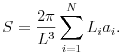
The specific internal surface on the other hand is given as
 |
(3.59) |
In a stochastic model
the radii ![]() and tube lengths
and tube lengths ![]() are chosen at random
according to a joint probability density
are chosen at random
according to a joint probability density ![]() .
.
Several special cases are of particular interest.
If the random radii ![]() and tube lengths
and tube lengths ![]() are chosen statistically
independently then the joint density
are chosen statistically
independently then the joint density ![]() factorizes as
factorizes as
![]() into a “pore width distribution”
into a “pore width distribution”
![]() and a “pore length distribution”
and a “pore length distribution” ![]() .
The average porosity and average specific internal surface area
become in this case
.
The average porosity and average specific internal surface area
become in this case
| (3.60) | ||||
| (3.61) |
where ![]() is the number of capillaries per unit area, and
is the number of capillaries per unit area, and
![]() is the average tortuosity factor obtained
by averaging the dimensionless tortuosity
is the average tortuosity factor obtained
by averaging the dimensionless tortuosity ![]() defined for each tube as
defined for each tube as
| (3.62) |
Moreover in this case the ratio
| (3.63) |
is a characteristic length independent of the tortuosity and
sample size.
Two further special cases arise from setting all radii equal
to each other, ![]() or all lengths equal to the system size,
or all lengths equal to the system size,
![]() .
If
.
If ![]() the tortuosity factor in (3.60) and
(3.61) is unity, and (3.63) holds
unchanged.
If the
the tortuosity factor in (3.60) and
(3.61) is unity, and (3.63) holds
unchanged.
If the ![]() are chosen statistically independently
then for large
are chosen statistically independently
then for large ![]() the average porosity is related to the
variance of the specific internal surface according to
the average porosity is related to the
variance of the specific internal surface according to
| (3.64) |
In the case where all radii are equal, ![]() , the relation
(3.63) simplifies to
, the relation
(3.63) simplifies to
| (3.65) |
Although this relation holds only in a special case it has become the basis for defining the so called hydraulic radius
| (3.66) |
as a characteristic length scale of porous media [1, 2]. The hydraulic radius concept was used in section III.A.3.d for defining pore size distributions. The capillary tube model and the hydraulic radius concept play an important role for fluid flow through porous media, and will be discussed further in section V.C.2 below.
A model which is closely related to the capillary tube model
is obtained by considering ![]() slits, i.e.
slits, i.e. ![]() parallel planes
of width
parallel planes
of width ![]() , instead of tubes.
All slits are assumed to be parallel and hence nonintersecting.
The resulting capillary slit model has a porosity
, instead of tubes.
All slits are assumed to be parallel and hence nonintersecting.
The resulting capillary slit model has a porosity
 |
(3.67) |
and specific internal surface area
| (3.68) |
independent of the widths of the slits. Here the specific internal surface is independent of the distribution of widths. As in the capillary tube model one finds a relation
| (3.69) |
similar to (3.65) also for the model of capillary slits. The model may be generalized by allowing small undulations and smooth fluctuations of the slits.
III.B.2 Grain Models
Grain models of various sorts have long been studied in optics
[193, 179], colloids [194, 195],
phase transitions [196] and disordered systems
[197].
An important class of grain models are random bead packs
[198, 199, 200, 201, 202, 203, 204] which provide a
reasonable starting point for modeling unconsolidated sediments.
In grain models either the pore or the matrix space are
represented as an array of convex grains
[205, 108, 109, 206, 207, 107, 208, 209].
The grains could be regularly shaped such as spheres,
cubes or ellipoids, or more irregularly shaped convex sets.
They may be positioned randomly or regularly in space, and
they may have equal or varying diameters.
If the grains are placed randomly their centroids are
assumed to form a stochastic point process.
For a Poisson point process the centers or centroids of
the grains are placed randomly and independently in space such
that the number ![]() of points inside a set
of points inside a set ![]() is Poisson
distributed with point density
is Poisson
distributed with point density ![]() .
For a Poisson point process the whole distribution is determined
by its density
.
For a Poisson point process the whole distribution is determined
by its density ![]() .
If
.
If ![]() are
are ![]() disjoint bounded sets then the
numbers
disjoint bounded sets then the
numbers ![]() are independent Poisson
random variables with joint probability distribution
are independent Poisson
random variables with joint probability distribution
| (3.70) |
The Poisson point process with constant density is stationary
and isotropic.
The contact distribution ![]() , defined in section
III.A.4, for the Poisson point process
can be obtained from the so called void probability that there
is no point inside
, defined in section
III.A.4, for the Poisson point process
can be obtained from the so called void probability that there
is no point inside ![]() as
as
| (3.71) |
A simple class of grain models is obtained by attaching compact
sets to the points of a Poisson point process.
The compact sets are called primary grains.
An example are spheres of constant radius.
Important generalizations are obtained by randomizing the primary
grains.
An example would be spherical grains with random radii.
More generally it is possible to use as grains independent
realizations of a random compact set as defined in section
II.B.2.b.
If ![]() denote the independent realizations of the grains and
denote the independent realizations of the grains and
![]() the points of a Poisson point process then a grain model
is obtained as the set
the points of a Poisson point process then a grain model
is obtained as the set
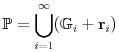 |
(3.72) |
if the grains are interpreted as pores.
If the grains are matrix then ![]() has to be replaced by
has to be replaced by ![]() .
The grain model is uniquely characterized by its capacity functional
.
The grain model is uniquely characterized by its capacity functional
![]() defined in section
III.A.6 above.
If
defined in section
III.A.6 above.
If ![]() denotes an independent realization of the primary grains,
and
denotes an independent realization of the primary grains,
and ![]() a compact set, then the capacity functional can be shown
to have the form [10, 37]
a compact set, then the capacity functional can be shown
to have the form [10, 37]
| (3.73) |
where ![]() denotes the expectation value with respect to
the distribution of primary grains, and the Minkowski addition
denotes the expectation value with respect to
the distribution of primary grains, and the Minkowski addition ![]() of sets was defined in (3.17).
The porosity of a grain model is obtained as
of sets was defined in (3.17).
The porosity of a grain model is obtained as
| (3.74) |
where ![]() is again a typical primary grain.
The covariance function defined in (3.7) and (3.8)
reads
is again a typical primary grain.
The covariance function defined in (3.7) and (3.8)
reads
| (3.75) |
and it determines the specific internal surface according to
(3.16) and (3.13).
The contact distribution ![]() for a compact set
for a compact set ![]() is given as
is given as
| (3.76) |
where the interior ![]() of a set was defined in
section II.B.1 and
of a set was defined in
section II.B.1 and ![]() .
.
Two simple classes of grain models are obtained by randomly
placing penetrable or impenetrable spheres of radius ![]() and
number density
and
number density ![]() .
Specializing (3.74) to spherical
grains of equal diameter one obtains
.
Specializing (3.74) to spherical
grains of equal diameter one obtains
| (3.77) |
for the porosity of fully penetrating spheres. The relation
| (3.78) |
applies to hard spheres of radius ![]() [108].
The specific internal surface area of overlapping spheres
reads
[108].
The specific internal surface area of overlapping spheres
reads
| (3.79) |
and for hard spheres
| (3.80) |
is obtained [108].
A basic question of stereology concerns the “unfolding” of
threedimensional information from planar sections [210].
For a stationary Poisson distributed grain model with spherical grains
of random diameter the problem of calculating the probability
density ![]() of the diameters of spheres from the probability
density
of the diameters of spheres from the probability
density ![]() of section circles was solved long ago
[211, 212].
The spatial and planar distributions are related through an
Abel integral equation
of section circles was solved long ago
[211, 212].
The spatial and planar distributions are related through an
Abel integral equation
| (3.81) |
where the mean sphere diameter ![]() is given by
is given by
![a=\frac{\pi}{2}\left[\int _{0}^{\infty}\frac{1}{r}p_{2}(r)dr\right]^{{-1}}.](mi/mi502.png) |
(3.82) |
The solution to this equation is
| (3.83) |
for ![]() .
In the special case where all spheres have the same constant diameter
.
In the special case where all spheres have the same constant diameter
![]() the probability density of section circle diameters is given as
the probability density of section circle diameters is given as
| (3.84) |
with ![]() .
The average diameter of the section circles is
.
The average diameter of the section circles is ![]() ,
and its variance is
,
and its variance is ![]() .
Another interesting special case is when the diameters of the
spheres are distributed according to
.
Another interesting special case is when the diameters of the
spheres are distributed according to
| (3.85) |
for ![]() which gives a mean sphere diameter
which gives a mean sphere diameter ![]() .
In this case the distribution reproduces itself, i.e
.
In this case the distribution reproduces itself, i.e
![]() .
.
Even the simplest grain model with penetrable spheres of equal
diameter and Poisson distributed centers still poses unsolved problems.
At low dimensionless densities ![]() the grains form isolated bounded sets.
Here
the grains form isolated bounded sets.
Here ![]() is the radius of the spheres and
is the radius of the spheres and ![]() their
number density.
As the dimensonless density is increased the grains begin to
overlap and ultimately “percolate” which means that an
unbounded connected component appears.
This continuum percolation transition between a state without
unbounded connected component and a state where the grains percolate
to infinity is a phase transition of order larger than two in the sense
of statistical mechanics [213, 64].
It continues to be the subject of much research in recent years
[214, 215, 216, 217, 218, 219].
their
number density.
As the dimensonless density is increased the grains begin to
overlap and ultimately “percolate” which means that an
unbounded connected component appears.
This continuum percolation transition between a state without
unbounded connected component and a state where the grains percolate
to infinity is a phase transition of order larger than two in the sense
of statistical mechanics [213, 64].
It continues to be the subject of much research in recent years
[214, 215, 216, 217, 218, 219].
A different parallel with statistical mechanics emerges if the grains are identified with the particles in statistical mechanics [6, 7, 8, 208]. This identification suggests generalizations of the underlying uncorrelated Poisson point process, which corresponds to an ideal gas of noninteracting particles, by adding interactions between the points. A large variety of new models such as hard sphere models or Gibbs point fields [37, 34] emerges from this generalization.
III.B.3 Network Models
Network models represent the most important and widely used class of geometric models for porous media [220, 221, 222, 223, 224, 225, 187, 226, 227, 228, 229, 230, 155, 157, 231, 232, 233]. They are not only used in theoretical calculations but also in the form of micromodels in experimental observations [157, 234, 235, 232, 236, 237, 238]. For random bead packs a random network model has recently been derived starting from the microstructure [204, 200]. Network models arise generally and naturally from discretizing the equations of motion using finite difference schemes. As such they will be discussed in more detail in chapter V.
A network is a graph consisting of a set of vertices or sites connected by a set of bonds. The vertices or sites of the network could for example represent the grain centers of a grain model. If the grains represent pore bodies the bonds represent connections between them. The vertices can be chosen deterministically as for the sites of a regular lattice or randomly as in the realization of a Poisson or other stochastic point process. Similarly the bonds connecting different vertices may be chosen according to some deterministic or random procedure. Finally the vertices are “dressed” with convex sets such as spheres representing pore bodies, and the bonds are dressed with tubes providing a connecting path between the pore bodies. A simple ordered network model consists of a regular lattice with spheres of equal radius centered at its vertices which are connected through cylindrical tubes of equal diameter. Very often the diameters of spheres and tubes in a regular network model are chosen at random. If a finite fraction of the bond diameters is zero one obtains the percolation model.
III.B.4 Percolation Models
The purpose of the present section is not to review percolation theory but to introduce the concept of a percolation transition, and to collect for later reference the values of percolation thresholds. The name “percolation” derives from fluid flow through a coffee percolator, and it has been used extensively to model various aspects of flow through porous media [239, 154, 41, 153, 156, 113, 240, 241, 242, 243, 226]. Invasion percolation has become a frequently studied model for displacement processes in porous media [244, 245, 246, 42, 246a]. Percolation theory itself is a well developed branch in the theory of disordered systems and critical phenomena, and the reader is referred to [247, 197, 248, 213] for thorough information on the subject.
Percolation as a geometrical model for porous media is closely related both to grain models and to network models. The model of spherical grains attached to the points of a Poisson process is also known as continuum percolation or the “swiss cheese” model [213]. Site percolation is an abstract version of a grain model, while bond percolation may be seen as an abstraction from network models. The distinguishing feature of percolation theory from other models is its focus on a sudden phase transition associated with the connectivity of random media.
The simplest model of percolation is bond percolation on
a lattice.
In bond percolation the bonds of a regular
(e.g. simple cubic) lattice are occupied randomly
with connecting (=conducting) elements ( e.g. tubes)
with a certain occupation probability ![]() .
Alternatively one removes a fraction
.
Alternatively one removes a fraction ![]() of bonds
at random from a fully occupied infinite lattice.
Two lattice sites are called connected if there
exists a path between them traversing only bonds
occupied by connecting elements.
A set of connected bonds is called a cluster.
In an infinitely large system there exists a critical
occupation probability
of bonds
at random from a fully occupied infinite lattice.
Two lattice sites are called connected if there
exists a path between them traversing only bonds
occupied by connecting elements.
A set of connected bonds is called a cluster.
In an infinitely large system there exists a critical
occupation probability ![]() above which there
exists an unbounded connected cluster, while below
above which there
exists an unbounded connected cluster, while below
![]() all clusters are finite and bounded.
If the connecting elements are cylindrical tubes of fixed
or variable diameter then the resulting network model of
a porous medium would be permeable above
all clusters are finite and bounded.
If the connecting elements are cylindrical tubes of fixed
or variable diameter then the resulting network model of
a porous medium would be permeable above ![]() and
impermeable below.
and
impermeable below.
Similarly site percolation may be viewed as a lattice
version of a grain model.
In site percolation the sites of the underlying regular lattice
are occupied randomly with spherical pore bodies of radius at least
half the lattice constant.
Two nearest neighbour sites are called connected if they are both
occupied.
As in bond percolation there exist a critical occupation
probability ![]() separating a permeable connected
regime from an impermeable regime.
separating a permeable connected
regime from an impermeable regime.
These basic bond and site percolation models may be modified in many ways. The underlying lattice may be replaced with an arbitrary regular or random graph. The radii of tubes and pores may be randomized, and the connectivity criterion may be changed. Table II shows the values of the critical occupation probabilities (thresholds) for bond and site percolation for some common two and three dimensional lattices [213]. The table lists also the coordination number of each lattice defined as the number of bonds meeting at an interior lattice site.
| Lattice Type | Dimension | Coordination | ||
|---|---|---|---|---|
| honeycomb | 2 | 3 | 0.6962 | |
| square | 2 | 4 | 1/2 | 0.592746 |
| triangular | 2 | 6 | 1/2 | |
| diamond | 3 | 4 | 0.3886 | 0.4299 |
| simple cubic | 3 | 6 | 0.2488 | 0.3116 |
| body centered cubic | 3 | 8 | 0.180 | 0.246 |
| face centered cubic | 3 | 12 | 0.119 | 0.198 |
The transition between the permeable regime and the impermeable
regime becomes a phase transition in the limit of an infinitely
large lattice.
The role of the order parameter is played by the percolation
probability ![]() defined as the probability that a given point belongs
to an infinite cluster.
The correlation length
defined as the probability that a given point belongs
to an infinite cluster.
The correlation length ![]() is defined from the correlation function
giving the probability that a site at distance
is defined from the correlation function
giving the probability that a site at distance ![]() from a given site
is occupied and connected to the given site.
The correlation length measures the typical size of a cluster, and
it diverges as
from a given site
is occupied and connected to the given site.
The correlation length measures the typical size of a cluster, and
it diverges as ![]() approaches
approaches ![]() .
.
III.B.5 Filtering and Reconstruction
Recently a new type of geometric models has appeared
[249, 250, 171, 251, 118, 252] which is
based on image processing techniques.
These models attempt to reconstruct a porous medium
with prespecified statistical characteristics such
as its porosity ![]() and two point correlation
function
and two point correlation
function ![]() [249, 250].
This is achieved through real space or Fourier space
filtering of random fields.
To this end a two or three dimensional random function
assigning an independent random number to each point
in space is convoluted with a smoothing kernel.
Alternatively the Fourier transforms of the two functions
are multiplied and backtransformed to obtain the smoothed
image.
In [249, 250, 252] it has been argued that such
reconstructed images resemble the structures observed in
sedimentary rocks or Vycor glass.
In [171] such models have been used to test the
microstructural sensitivity of local porosity distributions
(discussed above in section III.A.5) on
models with identical two point correlation functions.
[249, 250].
This is achieved through real space or Fourier space
filtering of random fields.
To this end a two or three dimensional random function
assigning an independent random number to each point
in space is convoluted with a smoothing kernel.
Alternatively the Fourier transforms of the two functions
are multiplied and backtransformed to obtain the smoothed
image.
In [249, 250, 252] it has been argued that such
reconstructed images resemble the structures observed in
sedimentary rocks or Vycor glass.
In [171] such models have been used to test the
microstructural sensitivity of local porosity distributions
(discussed above in section III.A.5) on
models with identical two point correlation functions.
The motivation for studying reconstructed porous media is to generate precisely known microgeometries whose transport properties can then be calculated numerically [249, 252]. As shown in [171] two media with the same porosity and correlation function may still show significant differencs in their geometric characteristics. More importantly, the porosity and two point correlation function are not sufficient to determine the connectivity of a medium. The connectivity controls the transport, and therefore it is unclear to what extent reconstructed porous media are useful for predicting transport or relaxation properties.
III.B.6 Process Models
The geometric models discussed in the previous sections do not account
for the fact that the pore space configuration is often the result of a
physical process.
This suggests the use of dynamic process models which
describe the formation of the porous medium.
While such models are employed routinely for unconsolidated
bead packs [201, 253, 199, 202] they are relatively rare
for consolidated porous media.
The so called bond shrinkage model [254] was developed
for sedimentary rocks.
In this model one starts from a random resistor network on a
simple cubic lattice in ![]() dimensions.
Each resistor in the model represents a cylindrical tube with
radius
dimensions.
Each resistor in the model represents a cylindrical tube with
radius ![]() in a corresponding network model on the lattice.
Next a tube element is randomly chosen and its radius is reduced
by a fixed factor
in a corresponding network model on the lattice.
Next a tube element is randomly chosen and its radius is reduced
by a fixed factor ![]() with
with ![]() .
The radius of the shrunk element is then
.
The radius of the shrunk element is then ![]() .
The shrinkage process may be repeated as often as necessary to
reach a specified porosity or until some other criterion is
satisfied depending on the modeling purpose.
The condition
.
The shrinkage process may be repeated as often as necessary to
reach a specified porosity or until some other criterion is
satisfied depending on the modeling purpose.
The condition ![]() guarantees that the model remains connected
at all times if the shrinkage is repeated a finite number of
times.
Because
guarantees that the model remains connected
at all times if the shrinkage is repeated a finite number of
times.
Because ![]() the bond shrinkage model does not give rise to
a percolation threshold.
the bond shrinkage model does not give rise to
a percolation threshold.
The so called grain consolidation model [255, 256]
does give rise to a percolation threshold.
In the grain consolidation model one starts from a grain model
with nonoverlapping grains ![]() .
The grains are then allowed to grow.
In the simplest version [255] the grains form a regular
cubic lattice of spheres.
As the grains grow the porosity is reduced and more and more
narrow constrictions between grains are closed.
Thus the system becomes impenetrable at a finite porosity.
For a regular simple cubic lattice of spheres the
percolation threshold appears at a critical porosity of
.
The grains are then allowed to grow.
In the simplest version [255] the grains form a regular
cubic lattice of spheres.
As the grains grow the porosity is reduced and more and more
narrow constrictions between grains are closed.
Thus the system becomes impenetrable at a finite porosity.
For a regular simple cubic lattice of spheres the
percolation threshold appears at a critical porosity of
![]() [255].
This value is much smaller than the values
[255].
This value is much smaller than the values ![]() or
or ![]() in Table II
for bond and site percolation.
If the grains are grown from a random bead pack the critical
porosity is found to be
in Table II
for bond and site percolation.
If the grains are grown from a random bead pack the critical
porosity is found to be ![]() .
This value is again much smaller than the threshold
.
This value is again much smaller than the threshold
![]() in continuum percolation [257, 258]
in continuum percolation [257, 258]
Another process model, called local porosity reduction model,
was introduced in [170].
Consider a simple regular lattice (e.g. simple cubic) with
lattice constant ![]() superimposed on a porous medium as shown
in Figure 12.
The lattice cells are the measurement cells of local porosity
theory defined in section III.A.5.
In the simplest example one may assume that all measurement
cells have the same initial porosity
superimposed on a porous medium as shown
in Figure 12.
The lattice cells are the measurement cells of local porosity
theory defined in section III.A.5.
In the simplest example one may assume that all measurement
cells have the same initial porosity ![]() and specific
internal surface area
and specific
internal surface area ![]() .
The consolidation process is modeled by picking at random
a particular cell and reducing its porosity by a factor
.
The consolidation process is modeled by picking at random
a particular cell and reducing its porosity by a factor ![]() ,
and its specific surface by a factor
,
and its specific surface by a factor ![]() .
This operation is repeated until a desired average porosity
.
This operation is repeated until a desired average porosity
![]() has been reached.
It is assumed that the local percolation probability function
has been reached.
It is assumed that the local percolation probability function
![]() is unaffected by the consolidation operations.
The final state of the porous medium can be described by
assigning to each cell the random integer
is unaffected by the consolidation operations.
The final state of the porous medium can be described by
assigning to each cell the random integer ![]() giving the
number of times a local consolidation operation was performed
on that cell.
The random variable
giving the
number of times a local consolidation operation was performed
on that cell.
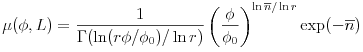
The random variable ![]() is Poisson distributed and this
observation allows to find the local porosity distribution
as [170]
is Poisson distributed and this
observation allows to find the local porosity distribution
as [170]
 |
(3.86) |
where
| (3.87) |
and ![]() denotes Eulers Gamma function.
A similar consideration could be performed for the specific
internal surface distribution.
In many consolidation processes the reduction factors are not
independent.
For grain consolidation models this is
illustrated by equations (3.77) through
(3.80) relating the porosity and
specific surface through the sphere radius.
Similarly, if a crack is closed by an applied external
pressure this will reduce the porosity but not the surface
area, as long as the possibility of crushing the crack profile
is neglected.
Therefore in this case
denotes Eulers Gamma function.
A similar consideration could be performed for the specific
internal surface distribution.
In many consolidation processes the reduction factors are not
independent.
For grain consolidation models this is
illustrated by equations (3.77) through
(3.80) relating the porosity and
specific surface through the sphere radius.
Similarly, if a crack is closed by an applied external
pressure this will reduce the porosity but not the surface
area, as long as the possibility of crushing the crack profile
is neglected.
Therefore in this case ![]() .
Similarly if a void space is uniformly cemented by precipitation
of minerals from the pore fluids this implies the relation
.
Similarly if a void space is uniformly cemented by precipitation
of minerals from the pore fluids this implies the relation
![]() between the reduction factors.
The simple relation
between the reduction factors.
The simple relation
| (3.88) |
summarizes several idealized processes such as
crack compaction, ![]() , shrinkage of capillaries,
, shrinkage of capillaries,
![]() , shrinkage of voids,
, shrinkage of voids, ![]() ,
and void filling,
,
and void filling, ![]() .
.
