III.A General Geometric Characterization Theories
A general geometric characterization of porous media should satisfy the following requirements:
-
It should be well defined in terms of geometric quantities.
-
It should involve only parameters which are directly observable or measurable in an experiment independent of the phenomenon of interest.
-
It should not require the specification of too many parameters. The required independent experiments should be simple and economical to carry out. What is economical depends on the available data processing technology. With current data processing technology a characterization requiring more than
 numbers must be considered
uneconomical.
numbers must be considered
uneconomical. -
The characterization should be usable in exact or approximate solutions of the equations of motion governing the phenomenon of interest.
The following sections discuss methods based on porosities ![]() ,
correlation functions
,
correlation functions ![]() , local porosity distributions
, local porosity distributions
![]() , pore size distributions
, pore size distributions ![]() and capacities
and capacities ![]() .
Table I collects the advantages and disadvantages
of these methods according to the specified criteria.
.
Table I collects the advantages and disadvantages
of these methods according to the specified criteria.
| Characterization | well defined | predictive | economical | easily usable |
|---|---|---|---|---|
| yes | yes | yes | yes | |
| yes | yes | yes | yes | |
| yes | yes | no | yes | |
| no | no | yes | yes | |
| yes | yes | yes | yes | |
| yes | no | no | no |
III.A.1 Porosity and Other Numbers
III.A.1.a Porosity
The porosity of a porous medium is its most important geometrical property. Most physical properties are influenced by the porosity.
The porosity ![]() of a two component porous medium
of a two component porous medium
![]() consisting of a pore space
consisting of a pore space ![]() (component one)
and a matrix space
(component one)
and a matrix space ![]() (component two) is defined as the ratio
(component two) is defined as the ratio
| (3.1) |
which gives the volume fraction of pore space.
Here ![]() denotes the volume of the pore space defined in
(2.3) and
denotes the volume of the pore space defined in
(2.3) and ![]() is the total sample volume.
In the following the shorthand notation
is the total sample volume.
In the following the shorthand notation ![]() will often be employed.
will often be employed.
The definition (3.1) is readily extended to
stochastic porous media.
In that case ![]() and
and ![]() are random variables.
If the medium is stationary then one finds using
(2.3) and (2.11)
are random variables.
If the medium is stationary then one finds using
(2.3) and (2.11)
| (3.2) | ||||
where the last line holds only if the medium is stationary.
![]() in the last line is an arbitrary point.
Although the use of the expectation value
in the last line is an arbitrary point.
Although the use of the expectation value ![]() from (2.11) requires an underlying discretization
a continuous notation was used to indicate that the result
holds also in the continuous case.
If the stochastic porous medium is not only stationary but
also mixing or ergodic, and if it can be thought
of as being infinitely extended, then the limit
from (2.11) requires an underlying discretization
a continuous notation was used to indicate that the result
holds also in the continuous case.
If the stochastic porous medium is not only stationary but
also mixing or ergodic, and if it can be thought
of as being infinitely extended, then the limit
| (3.3) |
exists and equals ![]() .
Here the diameter
.
Here the diameter ![]() of a set
of a set ![]() is defined as
is defined as
![]() as the
supremum of the distance between pairs of points.
The notation
as the
supremum of the distance between pairs of points.
The notation ![]() indicates a
spatial average while
indicates a
spatial average while ![]() is a configurational average.
is a configurational average.
Equation (3.3) represents always an idealization.
Geological porous media for example are often heterogeneous
on all scales [5].
This means that their composition or volume fraction
![]() does not approach a limit for
does not approach a limit for ![]() .
Equation (3.3) assumes the existence of a length
scale beyond which fluctuations of the porosity decrease.
This scale is used traditionally to define so called
“representative elementary volumes” [76, 5].
The problem of macroscopic heterogeneity is related to the
remarks in the disccusion of stationarity in section
II.B.2.
It will be taken up again in section III.A.5
below.
.
Equation (3.3) assumes the existence of a length
scale beyond which fluctuations of the porosity decrease.
This scale is used traditionally to define so called
“representative elementary volumes” [76, 5].
The problem of macroscopic heterogeneity is related to the
remarks in the disccusion of stationarity in section
II.B.2.
It will be taken up again in section III.A.5
below.
The definition of porosity in (3.1) gives the so called total porosity which has to be distinguished from the open porosity or effective porosity. Open porosity is the ratio of accessible pore volume to total volume. Accessible means connected to the surface of the sample.
The porosity of a simple porous medium ![]() is related to the
bulk density
is related to the
bulk density ![]() the density of the matrix material
the density of the matrix material
![]() and the density of the pore space material
and the density of the pore space material ![]() through
through
| (3.4) |
Therefore porosity is conveniently determined from measuring densities using liquid buoyancy or gas expansion porosimetry [3, 1, 77, 2]. Other methods of measuring porosity include small angle neutron, small angle X-ray scattering and quantitative image analysis for total porosity [2, 77, 78, 43, 44]. Open porosity may be obtained from Xylene and water impregnation, liquid metal impregnation, Nitrogen adsorption and air or Helium penetration [77, 44].
Porosity in rocks originates as primary porosity during sedimentation or organogenesis and as secondary porosity at later stages of the geological development [1]. In sedimentary rocks the porosity is further classified as intergranular porosity between grains, intragranular or intercrystalline porosity within grains, fracture porosity caused by mechanical or chemical processes, and cavernous porosity caused by organisms or chemical processes.
III.A.1.b Specific Internal Surface Area
Similar to the porosity the specific internal surface area is an important geometric characteristic of porous media. In fact, a porous medium may be loosely defined as a medium with a large “surface to volume” ratio. The specific internal surface area is a quantitative measure for the surface to volume ratio. Often this ratio is so large that it has been idealized as infinite [78, 43, 79, 80, 81, 82, 83, 84, 85] and the application of fractal concepts has found much recent attention [58, 86, 87, 88, 84, 42, 89, 90, 91]
The specific internal surface ![]() of a two component porous
medium is defined as
of a two component porous
medium is defined as
| (3.5) |
where ![]() is the surface area, defined in eq. (2.3),
of the boundary set
is the surface area, defined in eq. (2.3),
of the boundary set ![]() .
The surface area
.
The surface area ![]() exists only if the internal
surface or interface
exists only if the internal
surface or interface ![]() fulfills suitable smoothness
requirements.
Fractal surfaces would have
fulfills suitable smoothness
requirements.
Fractal surfaces would have ![]() and in such
cases it is necessary to replace the Lebesgue measure in
(2.3) with the Hausdorff measure or another
suitable measure of the “size” of
and in such
cases it is necessary to replace the Lebesgue measure in
(2.3) with the Hausdorff measure or another
suitable measure of the “size” of ![]() [58, 59, 60, 61].
[58, 59, 60, 61].
The specific internal surface is a characteristic inverse
length giving the surface to volume ratio of a porous medium.
Typical values for unconsolidated sand are ![]() m
m![]() ,
and range from
,
and range from ![]() m
m![]() to
to ![]() m
m![]() for sandstones
[92, 3]. A piece of sandstone measuring
for sandstones
[92, 3]. A piece of sandstone measuring ![]() cm
on each side and having a specific internal surface of
cm
on each side and having a specific internal surface of
![]() m
m![]() contains the same area as a sports
arena of dimensions
contains the same area as a sports
arena of dimensions ![]() m
m![]() m.
This illustrates the importance of surface effects
for all physical properties of porous media.
m.
This illustrates the importance of surface effects
for all physical properties of porous media.
Specific internal surface area can be measured by similar
techniques as porosity.
Some commonly employed methods are given in Figure 1
together with their ranges of applicability.
Particularly important methods are based on physisorption
isotherms [93, 94].
The interpretation of the BET-method [93] is restricted
to certain types of isotherms, and its interpretation requires
considerable care.
In particular, if micropores are present these will be filled
spontaneously and application of the BET-analysis will lead
to wrong results [44].
Other methods to determine ![]() measure the two point correlation
function. As discussed further in the next section the
specific internal surface area can for statistically homogeneous
media be deduced from the slope of the correlation function
at the origin [95].
measure the two point correlation
function. As discussed further in the next section the
specific internal surface area can for statistically homogeneous
media be deduced from the slope of the correlation function
at the origin [95].
III.A.2 Correlation Functions
Porosity and specific internal surface area are merely two numbers characterizing the geometric properties of a porous medium. Obviously these two numbers are not sufficient for a full statistical characterization of the system. A full characterization can be given in terms of multipoint correlation functions [96, 97, 98, 99, 100, 101, 102, 103, 104, 6, 105, 106, 107, 108, 109, 110, 111, 112, 8].
The average porosity ![]() of a stationary two component
porous medium is given by equation (3.2) as
of a stationary two component
porous medium is given by equation (3.2) as
| (3.6) |
in terms of the expectation value of the random variable ![]() taking the value
taking the value ![]() if the point
if the point ![]() lies in the pore space and
lies in the pore space and ![]() if not.
This is an example of a so called one-point function.
An example of a two-point function is the covariance function
if not.
This is an example of a so called one-point function.
An example of a two-point function is the covariance function
![]() defined as
the covariance of two random variables
defined as
the covariance of two random variables ![]() and
and
![]() at two points
at two points ![]() and
and ![]() ,
,
| (3.7) |
For a stationary medium the covariance function depends only on
the difference ![]() which allows to set
which allows to set ![]() without
loss of generality. This gives
without
loss of generality. This gives
| (3.8) |
Because ![]() it follows that
it follows that
![]() .
The correlation coefficient of two random variables
.
The correlation coefficient of two random variables ![]() and
and ![]() is in general defined as the ratio of the covariance cov
is in general defined as the ratio of the covariance cov![]() to the
two standard deviations of
to the
two standard deviations of ![]() and
and ![]() [73, 74].
It varies between
[73, 74].
It varies between ![]() and
and ![]() corresponding to complete correlation
or anticorrelation.
The covariance function is often normalized analogous to the
correlation coefficient by division with
corresponding to complete correlation
or anticorrelation.
The covariance function is often normalized analogous to the
correlation coefficient by division with ![]() to obtain the
two-point correlation function
to obtain the
two-point correlation function
| (3.9) |
An illustration of a two point correlation function can be seen
in Figure 14.
The porosity in (3.6) is an example of a moment function.
The general ![]() -th moment function is defined as
-th moment function is defined as
![S_{n}({\bf r}_{1},...,{\bf r}_{n})=\left\langle\prod _{{i=1}}^{n}\left[\chi\rule[-4.3pt]{0.0pt}{8.6pt}_{{\mathbb{P}}}({\bf r}_{i})\right]\right\rangle](mi/mi153.png) |
(3.10) |
where the average is defined in eq. (2.11) with respect to the probability density of microstructures given in eq. (2.10). The covariance function in (3.7) or (3.8) is an example of a cumulant function (also known as Ursell or cluster functions in statistical mechanics). The n-th cumulant function is defined as
![C_{n}({\bf r}_{1},...,{\bf r}_{n})=\left\langle\prod _{{i=1}}^{n}\left[\chi\rule[-4.3pt]{0.0pt}{8.6pt}_{{\mathbb{P}}}({\bf r}_{i})-\left\langle\chi\rule[-4.3pt]{0.0pt}{8.6pt}_{{\mathbb{P}}}({\bf r}_{i})\right\rangle\right]\right\rangle=\left\langle\prod _{{i=1}}^{n}\left[\chi\rule[-4.3pt]{0.0pt}{8.6pt}_{{\mathbb{P}}}({\bf r}_{i})-\left\langle\phi\right\rangle\right]\right\rangle](mi/mi141.png) |
(3.11) |
where the second equality assumes stationarity.
The cumulant functions are related to the moment functions.
For ![]() one has the relations
one has the relations
| (3.12) | ||||
| (3.13) | ||||
| (3.14) | ||||
The analogous moment functions may be defined for the matrix space
![]() by replacing
by replacing ![]() in all formulas with
in all formulas with ![]() ,
and they have been called
,
and they have been called ![]() -point matrix probability functions
[105, 107] or simply correlation functions [111]
From (3.10),(2.10) and (2.11)
the probabilistic meaning of the moment functions is found as
-point matrix probability functions
[105, 107] or simply correlation functions [111]
From (3.10),(2.10) and (2.11)
the probabilistic meaning of the moment functions is found as
| (3.15) |
Therefore ![]() is the probability that all the points
is the probability that all the points
![]() fall into the pore space.
fall into the pore space.
The case ![]() of the second moment is of particular interest.
If the pore space is stationary and isotropic then
of the second moment is of particular interest.
If the pore space is stationary and isotropic then
![]() and one has
and one has ![]() .
If the porous medium is also mixing then
.
If the porous medium is also mixing then ![]() .
If the pore space
.
If the pore space ![]() is three dimensional, and does not
contain flat twodimensional surfaces of zero thickness then
its derivative at the origin is related to the specific internal
surface area
is three dimensional, and does not
contain flat twodimensional surfaces of zero thickness then
its derivative at the origin is related to the specific internal
surface area ![]() through
through
| (3.16) |
In two dimensions an analogous formula holds in which ![]() is replaced
with a “specific internal length” and the denominator
is replaced
with a “specific internal length” and the denominator ![]() is replaced
with
is replaced
with ![]() .
.
The practical measurement of two point correlation functions
is based on Minkowski addition and subtraction of sets [10, 37].
The Minkowski addition of two sets ![]() and
and ![]() in
in ![]() is defined as the set
is defined as the set
| (3.17) |
Note that ![]() is the translation defined
in equation (2.17).
Therefore
is the translation defined
in equation (2.17).
Therefore
![]() is the union of the translates
is the union of the translates ![]() as
as ![]() runs through
runs through ![]() .
The dual operation to Minkowski addition is Minkowski subtraction
defined as
.
The dual operation to Minkowski addition is Minkowski subtraction
defined as
| (3.18) |
where ![]() denotes the complement of
denotes the complement of ![]() .
With these definitions the two-point function is given as
.
With these definitions the two-point function is given as
| (3.19) |
where ![]() is the set consisting of the origin
and the point
is the set consisting of the origin
and the point ![]() .
This formula is the basis for the statistical estimation of
.
This formula is the basis for the statistical estimation of ![]() and
and ![]() in image analysers from the area of the
“eroded” set
in image analysers from the area of the
“eroded” set ![]() .
The operation
.
The operation ![]() is called erosion
of the set
is called erosion
of the set ![]() with the set
with the set ![]() and it has been used in methods
to define pore size distributions which will be discussed in the
next section.
An example for the erosion of a pore space image by a set
and it has been used in methods
to define pore size distributions which will be discussed in the
next section.
An example for the erosion of a pore space image by a set ![]() is shown in Figure 9.
is shown in Figure 9.
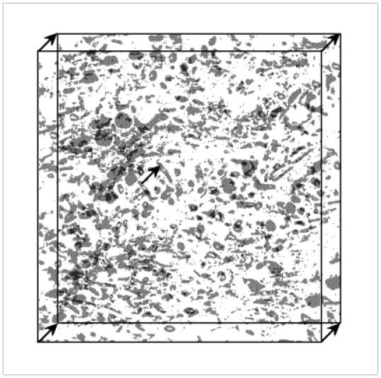
The original image (shown Figure 12) is obtained from
a cross section micrograph of a Savonnier oolithic sandstone.
Two copies of the image are displaced relative to each other
by a vector ![]() as indicated in Figure 9.
The two images are rendered in grey, and their intersection
is coloured black.
The area of the intersection is an estimate for
as indicated in Figure 9.
The two images are rendered in grey, and their intersection
is coloured black.
The area of the intersection is an estimate for ![]() .
.
The main advantage of the correlation function method for
characterizing porous media is that it provides a set of
well defined functions of increasing complexity for the
geometrical description.
In practice one truncates the hierarchy of correlation
functions at the two-point functions.
While this provides much more information about the geometry
than the porosity and specific surface area alone, many
important properties of the medium (such as its connectivity)
are buried in higher order functions.
2 (This is a footnote:) 2
Two points are called connected if there exists a path between
them which lies completely inside the pore space.
Therefore the probabilistic description of connectedness
properties requires multipoint correlation functions
involving all the points which make up the path.
Depending on the required accuracy a simple two point function
for a three dimensional stationary but anisotropic two
component medium could be specified by
![]() to
to ![]() data points which would be economical
according to the criterion adopted previously.
An
data points which would be economical
according to the criterion adopted previously.
An ![]() point function with the same accuracy
would require
point function with the same accuracy
would require ![]() to
to ![]() data points.
Specifying five or higher point functions
quickly becomes just as impractical as specifying a given
geometry completely.
data points.
Specifying five or higher point functions
quickly becomes just as impractical as specifying a given
geometry completely.
III.A.3 “Pore Size” Distributions
In certain porous materials such as wood (see Figure 5)
it is natural to identify cylindrically shaped pores and to
represent their disorder through a distribution of pore
diameters.
In other media such as systems with cavernous or oomoldic
porosity it is possible to identify roughly convex pore
bodies analogous to convex sand grains dispersed in
a uniform background.
If the radius ![]() of the cylindrical capillaries or
spherical pore bodies in such media is randomly distributed
then the pore size distribution function
of the cylindrical capillaries or
spherical pore bodies in such media is randomly distributed
then the pore size distribution function ![]() can be
defined as
can be
defined as
| (3.20) |
giving the probability that the random radius ![]() of the
cylinders or spheres is smaller than
of the
cylinders or spheres is smaller than ![]() .
For general porous microstructures, however, it is
difficult to define “pores” or “pore bodies”, and the
concept of pore size distribution remains ill defined.
.
For general porous microstructures, however, it is
difficult to define “pores” or “pore bodies”, and the
concept of pore size distribution remains ill defined.
Nevertheless many authors have introduced a variety of well defined probability distributions of length for arbitrary media which intended to overcome the stated difficulty [3, 2, 113, 114, 115, 116, 117, 118, 119]. The concept of pore size distributions enjoys continued popularity in most fields dealing with porous materials. Recent examples can be found in chromatography [120, 121], membranes [122, 123, 124], polymers [125], ceramics [126, 127, 128, 129], silica gels [130, 131, 132], porous carbon [133, 134], cements [135, 136, 137], rocks and soil science [138, 139, 140, 141, 142, 143], fuel research [144], separation and adhesion technology [30, 145] or food engineering [146]. The main reasons for this popularity are adsorption measurements [147, 30, 148] and mercury porosimetry [149, 150, 151, 152].
III.A.3.a Mercury Porosimetry
The “pore size distribution” of mercury porosimetry is not a geometric but a physical characteristic of a porous medium. Mercury porosimetry is a transport and relaxation phenomenon [43, 153], and its discussion would find a more appropriate place in chapter V below. On the other hand “pore size distributions” are routinely measured in practice using mercury porosimetry, and many readers will expect its discussion in a section on pore size distributions. Therefore pore size distributions from mercury porosimetry are discussed already here together with other definitions of this important concept.
Mercury porosimetry is based on the fact that mercury is a strongly
nonwetting liquid on most substrates, and that it has a high
surface tension.
To measure the “pore size distribution”
a porous sample ![]() with pore space
with pore space ![]() is evacuated inside
a pycnometer pressure chamber at elevated temperatures and low
pressures [43].
Subsequently the sample is immersed into mercury and
an external pressure is applied.
As the pressure is increased mercury is injected into
the pore space occupying a subset
is evacuated inside
a pycnometer pressure chamber at elevated temperatures and low
pressures [43].
Subsequently the sample is immersed into mercury and
an external pressure is applied.
As the pressure is increased mercury is injected into
the pore space occupying a subset ![]() of the
pore space which depends on the applied external pressure
of the
pore space which depends on the applied external pressure ![]() .
The experimenter records the injected volume of mercury
.
The experimenter records the injected volume of mercury
![]() as a function of the applied external pressure.
If the volume of the pore space
as a function of the applied external pressure.
If the volume of the pore space ![]() is known
independently then this gives the saturation
is known
independently then this gives the saturation
![]() as a function of pressure.
The cumulative “pore size” distribution function
as a function of pressure.
The cumulative “pore size” distribution function
![]() of mercury porosimetry is now
defined by
of mercury porosimetry is now
defined by
| (3.21) |
For rocks a contact angle ![]() and surface tension with vacuum of
and surface tension with vacuum of ![]() Nm
Nm![]() are commonly used [1, 43, 153].
The definition of
are commonly used [1, 43, 153].
The definition of ![]() is based on the equation
is based on the equation
| (3.22) |
for the capillary pressure ![]() which expresses the force
balance in a single cylindrcal capillary tube.
Equation (3.21) follows from (3.22)
if it is assumed that the saturation history
which expresses the force
balance in a single cylindrcal capillary tube.
Equation (3.21) follows from (3.22)
if it is assumed that the saturation history
![]() is identical to that obtained from
the so called capillary tube model discussed in section
III.B.1 below.
The capillary tube model is a hypothetical porous medium
consisting of parallel nonintersecting cylindrical capillaries
of random diameter.
is identical to that obtained from
the so called capillary tube model discussed in section
III.B.1 below.
The capillary tube model is a hypothetical porous medium
consisting of parallel nonintersecting cylindrical capillaries
of random diameter.
The fact that ![]() is not a geometrical quantity but a
capillary pressure function is obvious from its definition.
It depends on physical properties such as the nature of the
injected fluid or wetting properties of the walls.
For a suitable choice of tube diameter the function
is not a geometrical quantity but a
capillary pressure function is obvious from its definition.
It depends on physical properties such as the nature of the
injected fluid or wetting properties of the walls.
For a suitable choice of tube diameter the function ![]() of pressure could equally well be translated into a distribution
of the wetting angles
of pressure could equally well be translated into a distribution
of the wetting angles ![]() .
.
![]() shows hysteresis implying that the pore
size distribution
shows hysteresis implying that the pore
size distribution ![]() is process dependent.
is process dependent.
Although ![]() is not a geometrical quantity it contains
much useful information about the microstructure of the
porous sample.
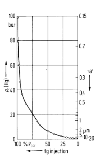
An example for the information obtained from mercury
porosimetry is shown in Figure 10 together with an image of the rock for which it
was measured [1].3 (This is a footnote:) 31 MPa = 10 bar = 10
is not a geometrical quantity it contains
much useful information about the microstructure of the
porous sample.
An example for the information obtained from mercury
porosimetry is shown in Figure 10 together with an image of the rock for which it
was measured [1].3 (This is a footnote:) 31 MPa = 10 bar = 10![]() dyn/cm
dyn/cm![]() = 9.869 atm = 145.04 psi
The rock is an example for a medium with hollow pores.
The correct interpretation of the saturation history
= 9.869 atm = 145.04 psi
The rock is an example for a medium with hollow pores.
The correct interpretation of the saturation history
![]() obtained from mercury porosimetry
continues to be an active research topic
[154, 155, 156, 157, 158, 159, 160].
obtained from mercury porosimetry
continues to be an active research topic
[154, 155, 156, 157, 158, 159, 160].
 |
 |
III.A.3.b Random Point Methods
Several authors [3, 113, 116] suggest to define
the “pore size” by first choosing a point ![]() at random
in the pore space, then to choose a compact set
at random
in the pore space, then to choose a compact set ![]() containing
containing
![]() , and finally to enlarge
, and finally to enlarge ![]() until it first intersects the
matrix space
until it first intersects the
matrix space ![]() .
In its simplest version [3, 116] the set
.
In its simplest version [3, 116] the set ![]() is
chosen as a small sphere
is
chosen as a small sphere ![]() of radius
of radius ![]() (see (2.5) above).
Then the pore size distribution
(see (2.5) above).
Then the pore size distribution ![]() of the random point
method is defined as the distribution function
of the random point
method is defined as the distribution function
![]() of the random
variable
of the random
variable ![]() defined as
defined as
| (3.23) |
Here ![]() is a random variable because
is a random variable because ![]() is chosen
at random.
is chosen
at random.
In a more sophisticated version of the same idea the set
![]() is chosen as a small coordinate cross whose axes
are then increased independently until they first touch
the matrix space. [113, 2].
This gives direction dependent pore size distributions.
is chosen as a small coordinate cross whose axes
are then increased independently until they first touch
the matrix space. [113, 2].
This gives direction dependent pore size distributions.
The main weakness of such a definition is that it is imprecise.
This becomes apparent from the fact that the randomness
of the pore sizes ![]() does not arise from the irregularities
of the pore space, but from the random placement of
does not arise from the irregularities
of the pore space, but from the random placement of ![]() .
Consider a regular pore space consisting of nonintersecting
spheres of equal radii
.
Consider a regular pore space consisting of nonintersecting
spheres of equal radii ![]() centered at the vertices
of a simple (hyper)cubic lattice.
Assuming that the points
centered at the vertices
of a simple (hyper)cubic lattice.
Assuming that the points ![]() are chosen at random
with a uniform distribution
it follows that the pore size distribution
are chosen at random
with a uniform distribution
it follows that the pore size distribution ![]() is not given by a
is not given by a ![]() -function at
-function at ![]() but
instead as a uniform distribution on the interval
but
instead as a uniform distribution on the interval
![]() .
More dramatically, exactly the same pore size distribution
is obtained for every pore space made from nonintersecting
spheres of equal radii, no matter whether they are placed
randomly or not.
In addition
.
More dramatically, exactly the same pore size distribution
is obtained for every pore space made from nonintersecting
spheres of equal radii, no matter whether they are placed
randomly or not.
In addition ![]() can be changed arbitrarily
by changing the distribution function governing the
random placement of
can be changed arbitrarily
by changing the distribution function governing the
random placement of ![]() .
.
III.A.3.c Erosion Methods
Another approach to the definition of a geometrical pore size
distribution [117, 118, 119] is borrowed from the
erosion operation in image processing [161, 162].
Erosion is defined in terms of Minkowski addition and subtraction
of sets introduced above in (3.17) and (3.18).
The erosion of a set ![]() by a set
by a set ![]() is defined as the
map
is defined as the
map ![]() .
The erosion was illustrated in Figure 9
for a pore space image and a set
.
The erosion was illustrated in Figure 9
for a pore space image and a set ![]() .
.
The method for locating “pore chambers”, “pore channels” and
“pore throats” suggested in [117] is based on eroding
the matrix space ![]() of a two component porous medium.
A ball
of a two component porous medium.
A ball ![]() is chosen as the structuring element.
The erosion
is chosen as the structuring element.
The erosion ![]() shrinks the matrix
space
shrinks the matrix
space ![]() .
The erosion operation is repeated until the matrix space
decomposes into disconnected fragments.
Continuing the erosion the pieces may either fragment again
or become convex.
If a piece becomes convex it is called a “grain”.
The centroid of the conves grain is called a “grain center”.
Reversing the erosion process allows to locate the point of
first/last contact of two fragments.
Connecting neighbouring grain centers by a path through
their last contact point produces a network model of the
grain space.
Having defined a network of grain centers and last contact
points the authors of [117], and their followers
[119, 118],
suggest to erect contact “surfaces” in each contact point.
A contact plane is defined as a “minimum area cross section”
of
.
The erosion operation is repeated until the matrix space
decomposes into disconnected fragments.
Continuing the erosion the pieces may either fragment again
or become convex.
If a piece becomes convex it is called a “grain”.
The centroid of the conves grain is called a “grain center”.
Reversing the erosion process allows to locate the point of
first/last contact of two fragments.
Connecting neighbouring grain centers by a path through
their last contact point produces a network model of the
grain space.
Having defined a network of grain centers and last contact
points the authors of [117], and their followers
[119, 118],
suggest to erect contact “surfaces” in each contact point.
A contact plane is defined as a “minimum area cross section”
of ![]() .
Subsequently a ball is placed at each grain center and
continually enlarged.
When the enlargement encounters a surface plane the
ball is truncated at the surface plane and only its
non-truncated pieces continue to grow until the sample
space is completely filled with the inflated grains.
The intersection points of three or more planes
in the resulting tesselation of space are defined
to be pore chambers.
The intersection lines of two planes are called
pore channels, and “minimal-area cross sections”
of the pore space
.
Subsequently a ball is placed at each grain center and
continually enlarged.
When the enlargement encounters a surface plane the
ball is truncated at the surface plane and only its
non-truncated pieces continue to grow until the sample
space is completely filled with the inflated grains.
The intersection points of three or more planes
in the resulting tesselation of space are defined
to be pore chambers.
The intersection lines of two planes are called
pore channels, and “minimal-area cross sections”
of the pore space ![]() along the pore channels are
called pore throats.
The pore throats are not unique, and sensitive to details
of the local geometry.
The pore chambers and the pore channels will in general
not lie in the pore space.
along the pore channels are
called pore throats.
The pore throats are not unique, and sensitive to details
of the local geometry.
The pore chambers and the pore channels will in general
not lie in the pore space.
A drawback of this procedure is that it is less unique than
it seems at first sight.
The network constructed from eroding the pore space is not unique
because the erosion operation involves the set ![]() as a
structuring element, and hence there are infinitely many
erosions possible.
The resulting grain network depends on the choice of the set
as a
structuring element, and hence there are infinitely many
erosions possible.
The resulting grain network depends on the choice of the set
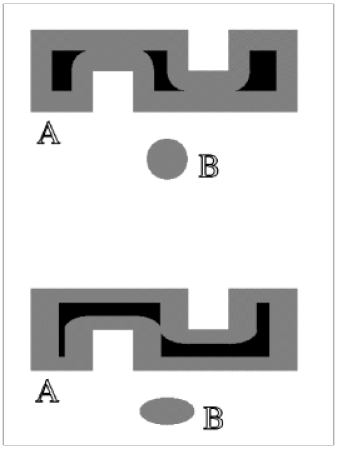
![]() , a fact which is not discussed in [117, 119].
Figure 11 shows an example where
erosion with a sphere produces three grains while
erosion with an ellipsoid produces only two grains.
The original set consists of the grey and black region,
the eroded part is coloured grey, and the residual set
is coloured black.
The theoretically described procedure for determining
the network was not carried out in practice [117].
Instead “subjective human preprocessing” ([117],p.4158)
was used to determine the network.
, a fact which is not discussed in [117, 119].
Figure 11 shows an example where
erosion with a sphere produces three grains while
erosion with an ellipsoid produces only two grains.
The original set consists of the grey and black region,
the eroded part is coloured grey, and the residual set
is coloured black.
The theoretically described procedure for determining
the network was not carried out in practice [117].
Instead “subjective human preprocessing” ([117],p.4158)
was used to determine the network.
III.A.3.d Hydraulic Radius Method
The hydraulic radius method [114, 115, 2]
for determining pore size distributions is based
on the idea of “symbolically closing pore throats”.
The definition of pore throats is given in terms of
“cross sections” of the pore space.
A cross section ![]() could be defined as the intersection
of a plane
could be defined as the intersection
of a plane ![]() , characterized by its unit normal
, characterized by its unit normal
![]() and a point
and a point ![]() in the plane, with
the pore space
in the plane, with
the pore space ![]() and some suitable set
and some suitable set ![]() which represents the region of interest and could depend on
the choice of plane.
In symbols
which represents the region of interest and could depend on
the choice of plane.
In symbols ![]() .
A pore throat containing the point
.
A pore throat containing the point ![]() is then
defined as
is then
defined as
| (3.24) |
where the minimum is taken over the unit sphere of orientations
of the planes.
A pore throat is now defined as a local minimum
of the function ![]() as
as ![]() is varied
over the pore space.
This ideal definition has in practice been replaced with
a subjective choice of orientations based on the assumption
of isotropy [114, 115, 2].
After constructing all pore throats of a medium the pore
space becomes divided into separate compartments called
“pore bodies” whose “size” can then be measured by
a suitable measure such as the volume to the power
is varied
over the pore space.
This ideal definition has in practice been replaced with
a subjective choice of orientations based on the assumption
of isotropy [114, 115, 2].
After constructing all pore throats of a medium the pore
space becomes divided into separate compartments called
“pore bodies” whose “size” can then be measured by
a suitable measure such as the volume to the power ![]() .
.
The definition of pore throats in hydraulic radius methods is very sensitive to surface roughness. This is readily seen from an idealized spherical pore with a few spikes. Another problem as remarked in [115], page 586, is that “the size of a pore body is not readily related in a unique manner to any measurable physical quantity”.
III.A.4 Contact and Chord Length Distributions
Chord length distributions [163, 164, 165, 166]
are special cases of so called contact distributions
[10, 37].
Consider the random matrix space ![]() of a two component stochastic
porous medium and choose a compact set
of a two component stochastic
porous medium and choose a compact set ![]() containing the origin
containing the origin ![]() .
Then the contact distribution is defined as the
conditional probability
.
Then the contact distribution is defined as the
conditional probability
| (3.25) | ||||
for ![]() .
Here
.
Here ![]() denotes the bulk porosity as usual.
Two special choices of the compact set
denotes the bulk porosity as usual.
Two special choices of the compact set ![]() are of
particular importance.
These are the unit sphere
are of
particular importance.
These are the unit sphere ![]() and the the unit
interval
and the the unit
interval ![]() .
.
For a unit sphere ![]() the quantity
the quantity
![]() is the conditional probability that a fixed point in the pore space
is the center of a sphere of radius
is the conditional probability that a fixed point in the pore space
is the center of a sphere of radius ![]() contained completely in the pore
space, under the condition that the chosen point does not belong to
contained completely in the pore
space, under the condition that the chosen point does not belong to ![]() .
If
.
If ![]() is isotropic and its boundary is sufficiently
smooth then the specific internal surface
is isotropic and its boundary is sufficiently
smooth then the specific internal surface ![]() can be obtained
from the derivative at the origin as [37]
can be obtained
from the derivative at the origin as [37]
| (3.26) |
The spherical contact distribution ![]() provides
a more precise formulation of the random point generation methods
for pore size distributions [3, 116] discussed in subsection
III.A.3.b.
provides
a more precise formulation of the random point generation methods
for pore size distributions [3, 116] discussed in subsection
III.A.3.b.
For the unit interval ![]() the contact distribution
the contact distribution
![]() is related to the chord length distribution
is related to the chord length distribution
![]() giving the probability that an interval in the
intersection of
giving the probability that an interval in the
intersection of ![]() with a straight line containing the unit
interval has a length smaller than
with a straight line containing the unit
interval has a length smaller than ![]() .
This provides a more precise formulation of the random point
generation ideas in [113, 2].
The relation between the contact distribution and the chord length
distribution is given by the equation
.
This provides a more precise formulation of the random point
generation ideas in [113, 2].
The relation between the contact distribution and the chord length
distribution is given by the equation
| (3.27) |
where the denominator on the right hand side gives the mean
chord length ![]() .
The mean chord length is related to the specific internal
surface area through
.
The mean chord length is related to the specific internal
surface area through ![]() .
In section III.A.2 it was mentioned that the specific
internal surface area can be obtained from the two point
function (see 3.16).
Therefore also the mean chord length can be related to
the correlation function through
.
In section III.A.2 it was mentioned that the specific
internal surface area can be obtained from the two point
function (see 3.16).
Therefore also the mean chord length can be related to
the correlation function through
| (3.28) |
Along these lines it has been suggested in [167] that the full chord length distribution can be obtained directly from small angle scattering experiments.
Contact and chord length distributions provide much more
geometrical information about the porous medium than the
porosity and specific surface area, and are at the same
time not as unnecessarily detailed as the complete
specification of the deterministic or stochastic
geometry.
Depending on the demands on accuracy a contact or chord
length distribution may be specified by 10 to 1000 numbers
irrespective of the microscopic resolution.
This should be compared with ![]() or
or ![]() numbers for a full deterministic or stochastic
characterization.
numbers for a full deterministic or stochastic
characterization.
III.A.5 Local Geometry Distributions
III.A.5.a Local Porosity Distribution
Local porosity distributions, or more generally local geometry distributions, provide a well defined general geometric characterization of stochastic porous media. [168, 169, 170, 171, 172, 173, 174, 175]. Local porosity distributions were mainly developed as an alternative to pore size distributions (see section III.A.3). They are intimately related with the theory of finite size scaling in statistical physics [176, 177, 64, 178]. Although fluctuations in the porosities have been frequently discussed [179, 10, 37, 2, 5, 180, 181, 76, 182], the concept of local porosity distributions and its relation with correlation functions was developed only recently [168, 169, 170, 171, 172, 173, 174, 175]. More applications are being developed [183, 184].
Local porosity distributions can be defined for deterministic
as well as for stochastic porous media.
For a single deterministic porous medium consider a partitioning
![]() of the sample space
of the sample space ![]() into
into ![]() mutually disjoint subsets, called measurement cells
mutually disjoint subsets, called measurement cells ![]() .
Thus
.
Thus ![]() and
and ![]() if
if ![]() .
A particular partitioning was used in the orginal
publications [178, 169, 170, 171]
where the
.
A particular partitioning was used in the orginal
publications [178, 169, 170, 171]
where the ![]() are unit cells centered at the vertices
of a Bravais lattice superimposed on
are unit cells centered at the vertices
of a Bravais lattice superimposed on ![]() .
This has the convenient feature that the
.
This has the convenient feature that the ![]() are
translated copies of one and the same set, and they all
have the same shape.
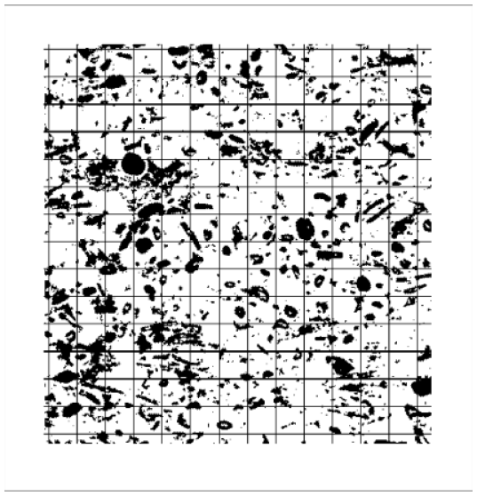
An example is illustrated in Figure 12 showing a
quadratic lattice as the measurement grid in two dimensions
superposed on a thin section of an oolithic sandstone.
are
translated copies of one and the same set, and they all
have the same shape.
An example is illustrated in Figure 12 showing a
quadratic lattice as the measurement grid in two dimensions
superposed on a thin section of an oolithic sandstone.
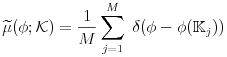
The local porosity inside a measurement cell ![]() is
defined as
is
defined as
![\phi(\mathbb{K}_{j})=\frac{V(\mathbb{P}\cap\mathbb{K}_{j})}{V(\mathbb{K}_{j})}=\frac{1}{M_{j}}\sum _{{{\bf r}_{i}\in\mathbb{K}_{j}}}\chi\rule[-4.3pt]{0.0pt}{8.6pt}_{{\mathbb{P}}}({\bf r}_{i})](mi/mi176.png) |
(3.29) |
where the second equality applies in case of discretized space
and ![]() denotes the number of volume elements or voxels in
denotes the number of volume elements or voxels in ![]() .
Thus the empirical one cell local porosity density function
is defined as
.
Thus the empirical one cell local porosity density function
is defined as
 |
(3.30) |
where ![]() is the Dirac
is the Dirac ![]() -distribution.
Obviously the distribution depends on the choice of partitioning
the sample space.
Two extreme partitions are of immediate interest.
The first arises from setting
-distribution.
Obviously the distribution depends on the choice of partitioning
the sample space.
Two extreme partitions are of immediate interest.
The first arises from setting ![]() and thus each
and thus each
![]() contains only one individual volume element
contains only one individual volume element ![]() with
with ![]() .
In this case
.
In this case ![]() or
or ![]() depending on whether
the volume element falls into matrix space (0), or pore space (1).
This gives immediately
depending on whether
the volume element falls into matrix space (0), or pore space (1).
This gives immediately
| (3.31) |
where ![]() is the total porosity.
The other extreme arises for
is the total porosity.
The other extreme arises for ![]() and thus
and thus ![]() the
measurment cell coincides with the sample space.
In this case obviously
the
measurment cell coincides with the sample space.
In this case obviously
| (3.32) |
Note that in both extreme cases the local porosity density is completely
determined by the total porosity ![]() , which equals
, which equals
![]() if the sample is sufficiently large
and mixing or ergodicity (3.3) holds.
if the sample is sufficiently large
and mixing or ergodicity (3.3) holds.
For a stochastic porous medium the one cell local porosity density function is defined for each measurement cell as
| (3.33) |
where ![]() is an element of the partitioning of the
sample space.
For the finest partition with
is an element of the partitioning of the
sample space.
For the finest partition with ![]() and
and ![]() one
finds now using eq. (3.2)
one
finds now using eq. (3.2)
| (3.34) | ||||
independent of ![]() .
If mixing (3.3) holds then
.
If mixing (3.3) holds then ![]() if the sample becomes sufficiently large, and the result
becomes identical to equation (3.31) for deterministic
media.
In the other extreme of the coarsest partition one finds
if the sample becomes sufficiently large, and the result
becomes identical to equation (3.31) for deterministic
media.
In the other extreme of the coarsest partition one finds
| (3.35) |
which may in general differ from (3.32) even if
the sample becomes sufficiently large, and mixing holds.
This is an important observation because it emphasizes the
necessity to consider more carefully the infinite volume
limit ![]() .
.
If a large deterministic porous medium is just a realization
of a stochastic medium obeying the mixing property, and if the
![]() are chosen such that the random variables
are chosen such that the random variables ![]() are independent, then Gliwenkos theorem
[185] of mathematical statistics guarantees that the
empirical one cell distribution approaches
are independent, then Gliwenkos theorem
[185] of mathematical statistics guarantees that the
empirical one cell distribution approaches ![]() in the limit
in the limit ![]() . In symbols
. In symbols
| (3.36) |
where the right hand side is independent of the choice of ![]() .
Therefore
.
Therefore ![]() and
and ![]() are identified in the
following.
This identification emerges also from considering average
and variance as shown next.
are identified in the
following.
This identification emerges also from considering average
and variance as shown next.
Define the average local porosity
![]() as
the first moment of the local porosity distribution.
For a stationary (=homogeneous) porous medium the definitions
(3.33) and (3.29) immediately yield
as
the first moment of the local porosity distribution.
For a stationary (=homogeneous) porous medium the definitions
(3.33) and (3.29) immediately yield
| (3.37) | ||||
![\displaystyle\frac{1}{M_{j}}\sum _{{{\bf r}_{i}\in\mathbb{K}_{j}}}\left\langle\chi\rule[-4.3pt]{0.0pt}{8.6pt}_{{\mathbb{P}}}({\bf r}_{i})\right\rangle](mi/mi203.png) |
||||
where ![]() is a measurement cell.
Similarly, the variance of local porosities reads
is a measurement cell.
Similarly, the variance of local porosities reads
| (3.38) | ||||
![\displaystyle\frac{1}{M_{j}^{2}}\left\langle\right[M_{j}\phi-\sum _{{i=1}}^{{M_{j}}}\chi\rule[-4.3pt]{0.0pt}{8.6pt}_{{\mathbb{P}}}({\bf r}_{i})\left]{}^{2}\right\rangle](mi/mi202.png) |
||||
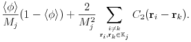 |
This result is important for two reasons.
Firstly it relates local porosity distributions to correlation
functions discussed above in section III.A.2.
Secondly it shows that the variance depends inversely on
the volume ![]() of the measurement cell.
This observation reconciles eq. (3.35) for stochastic
media with eq. (3.32) for deterministic media
because it shows that
of the measurement cell.
This observation reconciles eq. (3.35) for stochastic
media with eq. (3.32) for deterministic media
because it shows that ![]() approaches a degenerate
approaches a degenerate
![]() -distribution in the limit
-distribution in the limit ![]() .
Together with (3.37) and
.
Together with (3.37) and ![]() and
and ![]() for
for
![]() this shows that (3.35) and (3.32)
become equivalent.
this shows that (3.35) and (3.32)
become equivalent.
The ![]() -cell local porosity density function
-cell local porosity density function
![]() is the probability
density to find local porosity
is the probability
density to find local porosity ![]() in measurement cell
in measurement cell
![]() ,
, ![]() in
in ![]() and so on until
and so on until ![]() .
Formally it is defined by generalizing (3.33) to read
.
Formally it is defined by generalizing (3.33) to read
| (3.39) |
where the sets ![]() are a subset of measurement
cells in the partition
are a subset of measurement
cells in the partition ![]() .
Note that the
.
Note that the ![]() -cell functions
-cell functions ![]() are only defined for
are only defined for ![]() ,
i.e. if there are sufficient number of cells.
In particular for the extreme case
,
i.e. if there are sufficient number of cells.
In particular for the extreme case ![]() only the one-cell
function is defined.
In the extreme case
only the one-cell
function is defined.
In the extreme case ![]() of highest resolution (
of highest resolution (![]() )
the moments of the
)
the moments of the ![]() -cell local porosity distribution reproduce
the moment functions (3.10) of the correlation function
approach (section III.A.2) as
-cell local porosity distribution reproduce
the moment functions (3.10) of the correlation function
approach (section III.A.2) as
| (3.40) | ||||
where ![]() must be fulfilled.
This provides a connection between local porosity approaches
and correlation function approaches.
Simultaneously it shows
that the local porosity distributions are significantly
more general than correlation functions.
Already the one-cell function
must be fulfilled.
This provides a connection between local porosity approaches
and correlation function approaches.
Simultaneously it shows
that the local porosity distributions are significantly
more general than correlation functions.
Already the one-cell function ![]() contains more information
than the two-point correlation functions
contains more information
than the two-point correlation functions ![]() or
or ![]() as demonstrated on test images in [171].
as demonstrated on test images in [171].
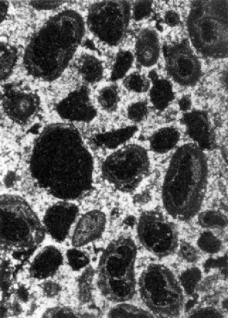
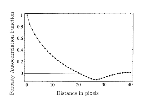
The most important practical aspect of local porosity distributions is that they are easily measurable in an independent experiment. Experimental determinations of local porosity distributions have been reported in [186, 173, 174, 175]. They were obtained from two dimensional sections through a sample of sintered glass beads. An example from [175] is shown in Figure 13.
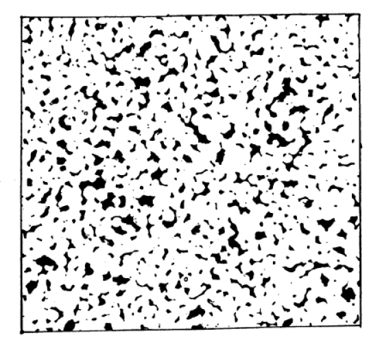
The porousmedium was made from sintering glass beads
of roughly ![]() m diameter.
Scanning electron migrographs obtained from the
specimen were then digitized with a spatial
resolution of
m diameter.
Scanning electron migrographs obtained from the
specimen were then digitized with a spatial
resolution of ![]() m per pixel.
The pore space is represented black in Figure
13 and the total porosity is
m per pixel.
The pore space is represented black in Figure
13 and the total porosity is ![]() .
The pixel-pixel correlation function of the pore space
image is shown in Figure 14.
.
The pixel-pixel correlation function of the pore space
image is shown in Figure 14.
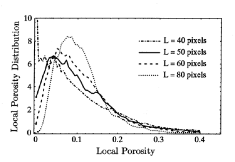
The local porosity distribution was then measured using
a square lattice with lattice constant ![]() .
The results are shown in Figure 15 for
measurement cell sizes of
.
The results are shown in Figure 15 for
measurement cell sizes of ![]() and
and ![]() pixels.
pixels.
Measurements of the local porosity distribution from three dimensional pore space images are currently carried out [183]. The pore space is reconstructed from serial sections which is a standard, but costly, technique to obtain threedimensional pore space representations [162, 187, 117, 113, 188, 114, 2, 183]. The advent of synchrotron microtomography [119, 4] and laser scanning confocal microscopy [188a] promises to reduce the cost and effort.
III.A.5.b Local Geometry Entropies
The linear extension ![]() of the measurement cells is
the length scale at which the pore space geometry is described.
The length
of the measurement cells is
the length scale at which the pore space geometry is described.
The length ![]() can be taken as the side length of a hypercubic
measurement cell, or more generally as the diameter
can be taken as the side length of a hypercubic
measurement cell, or more generally as the diameter
![]() of a cell
of a cell ![]() defined as the supremum of the distance
between pairs of points.
As
defined as the supremum of the distance
between pairs of points.
As ![]() the local porosity distribution
approaches a
the local porosity distribution
approaches a ![]() -distribution concentrated
at
-distribution concentrated
at ![]() according to (3.32) and (3.35).
For
according to (3.32) and (3.35).
For ![]() on the other hand it approaches two
on the other hand it approaches two ![]() -distributions
concentrated at
-distributions
concentrated at ![]() and
and ![]() according to (3.31) and
(3.34).
In both limits the local porosity distribution contains only
the bulk porosity
according to (3.31) and
(3.34).
In both limits the local porosity distribution contains only
the bulk porosity ![]() as a
geometric parameter.
At intermediate scales the distribution contains additional
information, such as the variance of the porosity fluctuations.
This suggests to search for an intermediate scale
as a
geometric parameter.
At intermediate scales the distribution contains additional
information, such as the variance of the porosity fluctuations.
This suggests to search for an intermediate scale
![]() which provides an optimal description.
Several criteria for determining
which provides an optimal description.
Several criteria for determining ![]() were discussed in
[171].
One interesting possibility is to optimize an information
measure or entropy associated with
were discussed in
[171].
One interesting possibility is to optimize an information
measure or entropy associated with ![]() , and
to define the entropy function
, and
to define the entropy function
| (3.41) |
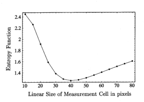
relative to the conventional a priori uniform distribution. The so called entropy length is then obtained from the extremality condition
| (3.42) |
That the entropy length ![]() exists and is well
defined was first demonstrated in [171]
using synthetic computer generated images.
Figure 16 shows the function
exists and is well
defined was first demonstrated in [171]
using synthetic computer generated images.
Figure 16 shows the function ![]() calculated for the image displayed in Figure 13.
A clear minimum appears at
calculated for the image displayed in Figure 13.
A clear minimum appears at ![]() pixels
corresponding to
pixels
corresponding to ![]() m.
m.
III.A.5.c Local Specific Internal Surface Distributions
Local specific internal surface area distributions are a
natural generalization of local porosity ditributions which
was first introduced in [171] in the
study of fluid transport in porous media.
Define the local specific internal surface area
in a cell ![]() as
as
![S(\mathbb{K}_{j})=\frac{V_{2}(\partial\mathbb{P}\cap\mathbb{K}_{j})}{V_{3}(\mathbb{K}_{j})}=\frac{1}{M_{j}}\sum _{{{\bf r}_{i}\in\mathbb{K}_{j}}}\chi\rule[-4.3pt]{0.0pt}{8.6pt}_{{\partial\mathbb{P}}}({\bf r}_{i})](mi/mi146.png) |
(3.43) |
which is analogous to equation (3.29). Generalizing equations (3.30) and (3.33) the local specific internal surface area probability density is defined as
| (3.44) |
in analogy with equation (3.33).
The joint probability density
![]() to find a local porosity
to find a local porosity
![]() and local specific internal surface
area in the range
and local specific internal surface
area in the range ![]() to
to ![]() and
and ![]() to
to ![]() will be called
local geometry distribution and it
is defined as the probability density
will be called
local geometry distribution and it
is defined as the probability density
| (3.45) |
The average specific internal surface area in a measurement
region ![]() is then obtained from the local geometry distribution as
is then obtained from the local geometry distribution as
| (3.46) |
and it represents an important local length scale.
Of course local geometry distributions can be extended to include other well defined geometric characteristics such as mean curvature or topological invariants. The definition of the generalized local geometry distribution is then obtained by generalizing (3.45).
III.A.5.d Local Percolation Probability
In addition to the local porosity distributions and local specific internal surface area distributions it is necessary to characterize the geometrical connectivity properties of a porous medium. This is important for discussing transport properties which depend critically on the connectedness of the pore space, but are less sensitive to its overall porosity or specific internal surface.
Two points inside the pore space ![]() of a two
component porous medium are called connected
if there exists a path contained entirely within
the pore space which connects the two points.
Using this connectivity criterion a cubic
measurement cell
of a two
component porous medium are called connected
if there exists a path contained entirely within
the pore space which connects the two points.
Using this connectivity criterion a cubic
measurement cell ![]() is called percolating if
there exist two points on opposite surfaces of
the cell which are connected to each other.
The local percolation probability
is called percolating if
there exist two points on opposite surfaces of
the cell which are connected to each other.
The local percolation probability ![]() is defined as the probability to find a percolating
geometry in measurement cells
is defined as the probability to find a percolating
geometry in measurement cells ![]() whose local
porosity is
whose local
porosity is ![]() and whose local specific internal
surface area is
and whose local specific internal
surface area is ![]() .
In practice the estimator for
.
In practice the estimator for ![]() is the fraction of percolating measurement cells which
have the prescribed values of
is the fraction of percolating measurement cells which
have the prescribed values of ![]() and
and ![]() .
.
III.A.5.e Large Scale Local Porosity Distributions
This section reviews the application of recent results in
statistical physics
[190, 63, 64, 65, 178, 66, 67, 68, 69]
to the problem of describing the
macroscopic heterogeneity on all scales.
The original definition (3.33) of the local porosity
distributions depends upon the size and shape of the
measurement cells, respectively on the partitioning ![]() of the sample space.
This dependence on the choice of a test set or “structuring
element” is characteristic for many methods of mathematical
morphology [10, 37, 71], and many of those discussed
in sections III.A.3 and III.A.4 above.
On the other hand subsection III.A.5.a
has shown that in the limit of large measurement cells
of the sample space.
This dependence on the choice of a test set or “structuring
element” is characteristic for many methods of mathematical
morphology [10, 37, 71], and many of those discussed
in sections III.A.3 and III.A.4 above.
On the other hand subsection III.A.5.a
has shown that in the limit of large measurement cells ![]() the form of the local porosity distribution
the form of the local porosity distribution ![]() becomes independent of
becomes independent of ![]() and approaches one and the same
universal limit given by
and approaches one and the same
universal limit given by ![]() .
This behaviour is an expression of the central limit theorem.
Local porosity distributions have support in the unit interval,
hence their second moment is always finite, and average local
porosities must become sharp in the limit.
It will be seen now that this behaviour is indeed
characteristic for macroscopically homogeneous
porous media, while other limiting distributions may
arise for macroscopically heterogeneous media.
.
This behaviour is an expression of the central limit theorem.
Local porosity distributions have support in the unit interval,
hence their second moment is always finite, and average local
porosities must become sharp in the limit.
It will be seen now that this behaviour is indeed
characteristic for macroscopically homogeneous
porous media, while other limiting distributions may
arise for macroscopically heterogeneous media.
Consider a convex measurement cell ![]() of volume
of volume ![]() .
Let
.
Let ![]() be the random scale factor at which the pore space
volume
be the random scale factor at which the pore space
volume ![]() of the inflated measurement
cell
of the inflated measurement
cell ![]() first exceeds
first exceeds ![]() , i.e. define
, i.e. define ![]() as
as
| (3.48) |
Consider ![]() mutually disjoint measurement cells
mutually disjoint measurement cells ![]()
![]() all having the same volume
all having the same volume ![]() .
Let
.
Let ![]() denote the scale factors associated with the
cells, and let
denote the scale factors associated with the
cells, and let ![]() be the
be the ![]() values
of the pore space volumes.
If the medium is homogeneous there exists a finite
correlation length beyond which fluctuations decrease.
Then the nonoverlapping cells
values
of the pore space volumes.
If the medium is homogeneous there exists a finite
correlation length beyond which fluctuations decrease.
Then the nonoverlapping cells ![]() can be chosen
such that the inflated cells remain nonoverlapping,
and such that they are separated more than the
correlation length.
Then the
can be chosen
such that the inflated cells remain nonoverlapping,
and such that they are separated more than the
correlation length.
Then the ![]() local porosities
local porosities ![]() are uncorrelated random variables.
For macroscopically heterogeneous media the correlation
length may be infinite, and thus it is necessary to
consider the limit
are uncorrelated random variables.
For macroscopically heterogeneous media the correlation
length may be infinite, and thus it is necessary to
consider the limit ![]() of infinitely large
cells to obtain uncorrelated porosities.
In [190, 63, 64, 65, 178]
the resulting ensemble limit
of infinitely large
cells to obtain uncorrelated porosities.
In [190, 63, 64, 65, 178]
the resulting ensemble limit ![]() has been defined and studied in detail.
In the present context the ensemble limit can be
used to study the limiting distribution of the
N-cell porosity
has been defined and studied in detail.
In the present context the ensemble limit can be
used to study the limiting distribution of the
N-cell porosity
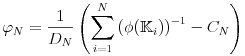
![\phi(\mathbb{K}_{1},...,\mathbb{K}_{N})=\frac{NV_{0}}{V_{1}+...+V_{N}}=N\left[\sum _{{i=1}}^{N}\left(\phi(\mathbb{K}_{i})\right)^{{-1}}\right]^{{-1}}](mi/mi175.png) |
(3.49) |
obtained from the ![]() measurements.
In the ensemble limit the
measurements.
In the ensemble limit the ![]() porosities
porosities ![]() become independent but ill defined, and this suggests to
consider instead the limiting behaviour of the
renormalized sums of positive random variables
become independent but ill defined, and this suggests to
consider instead the limiting behaviour of the
renormalized sums of positive random variables
 |
(3.50) |
where ![]() and
and ![]() are renormalization constants.
Note that
are renormalization constants.
Note that ![]() for all
for all ![]() .
.
If the sequence of distribution functions of the
random variables ![]() converges in the ensemble
limit
converges in the ensemble
limit ![]() and
and ![]() then the limiting distribution
is given by a stable law [74].
The existence of this limit is an indication of
fractional stationarity
[63, 64, 65, 178, 68, 69].
The limiting probability density function
for the variables
then the limiting distribution
is given by a stable law [74].
The existence of this limit is an indication of
fractional stationarity
[63, 64, 65, 178, 68, 69].
The limiting probability density function
for the variables ![]() is obtained
along the lines of [64] as
is obtained
along the lines of [64] as
| (3.51) |
where ![]() and the parameters obey the
restrictions
and the parameters obey the
restrictions ![]() ,
, ![]() and
and ![]() .
The function
.
The function ![]() appearing on the left hand
side is a generalized hypergeometric function which
can be defined through a Mellin-Barnes contour integral
[191].
The limiting local porosity density is obtained as the
distribution of the random variable
appearing on the left hand
side is a generalized hypergeometric function which
can be defined through a Mellin-Barnes contour integral
[191].
The limiting local porosity density is obtained as the
distribution of the random variable ![]() ,
and reads
,
and reads
| (3.52) |
for ![]() and
and ![]() for
for ![]() .
The universal limiting local porosity distributions
.
The universal limiting local porosity distributions
![]() depend on only three parameters,
and are independent of the diameter or size of the
measurement cells
depend on only three parameters,
and are independent of the diameter or size of the
measurement cells ![]() .
It is plausible that the limiting distributions
will also be independent of the shape of the measurement
cells, at least for the classes and sequences of convex
measurement sets usually employed in studying the
thermodynamic limit [192].
.
It is plausible that the limiting distributions
will also be independent of the shape of the measurement
cells, at least for the classes and sequences of convex
measurement sets usually employed in studying the
thermodynamic limit [192].
Because the limiting distributions have their support in
the interval ![]() all its moment exist,
and one has
all its moment exist,
and one has ![]() .
If the moments for
.
If the moments for ![]() can be inverted then
the parameters
can be inverted then
the parameters ![]() can be written as
can be written as
| (3.53) |
in terms of the first three integer moments.
Figure 17 displays
the form of ![]() for various values
of
for various values
of ![]() .
.

In the limit of small porosities ![]() the
result (3.52) behaves as a power law
the
result (3.52) behaves as a power law
| (3.54) |
Within local porosity theory this behaviour can give rise
to scaling laws in transport and relaxation properties of
porous media [170].
The importance of universal limiting local geometry
distributions arises from the fact that there exists a class
of limit laws which remains broad even after taking the
macroscopic limit ![]() .
This is the signature of macroscopic heterogeneity,
and it occurs for
.
This is the signature of macroscopic heterogeneity,
and it occurs for ![]() .
Macroscopically homogeneous systems, corresponding to
.
Macroscopically homogeneous systems, corresponding to
![]() , converge instead towards a
, converge instead towards a ![]() -distribution
concentrated at the bulk porosity
-distribution
concentrated at the bulk porosity ![]() .
.
III.A.6 Capacities
While local porosity distributions (in their one cell form) give a useful practical characterization of stochastic porous media they do not characterize the medium completely. A complete characterization of a stochastic medium is given by the so called Choquet capacities [72, 10]. Although this characterization is very important for theoretical and conceptual purposes it is not practical because it requires to specify the set of “all” compact subsets (see discussion in section II.B.2).
Consider the pore space ![]() of a stochastic two component porous
medium as a random set.
Let
of a stochastic two component porous
medium as a random set.
Let ![]() denote the family of all closed sets and
denote the family of all closed sets and ![]() the set
of all compact sets as in section II.B.2 above.
For any
the set
of all compact sets as in section II.B.2 above.
For any ![]() the “hitting function” or capacity
functional is defined as
the “hitting function” or capacity
functional is defined as
| (3.55) |
where Pr is the probability law governing the random set
![]() .
Then
.
Then ![]() has the following properties:
(i)
has the following properties:
(i) ![]() and
and ![]() .
(ii) If
.
(ii) If ![]() is a sequence of compact
subsset then
is a sequence of compact
subsset then ![]() implies
implies ![]() .
(iii) For all
.
(iii) For all ![]() the numbers
the numbers ![]() are
nonnegative where the
are
nonnegative where the ![]() are determined by the recursion
relation
are determined by the recursion
relation
| (3.56) |
and ![]() .
The number
.
The number ![]() gives the probability
that
gives the probability
that ![]() is empty, but
is empty, but ![]() is not empty
for all
is not empty
for all ![]() .
The functional
.
The functional ![]() is called an alternating Choquet capacity
of infinite order[10, 71].
is called an alternating Choquet capacity
of infinite order[10, 71].
Choquet’s theorem says that the converse is also true.
Explicitly, if ![]() is a functional on
is a functional on ![]() , then there exists
a necessarily unique distribution Pr in
, then there exists
a necessarily unique distribution Pr in ![]() with
with
| (3.57) |
for all ![]() if and only if
if and only if ![]() is an alternating Choquet
capacity of infinite order.
This theorem shows that capacity functionals play the same
defining role for random sets in continuous space as do the
numbers
is an alternating Choquet
capacity of infinite order.
This theorem shows that capacity functionals play the same
defining role for random sets in continuous space as do the
numbers ![]() in (2.10) in the
discrete case.
in (2.10) in the
discrete case.
The main problem with this theoretically important result
is that the family of hitting sets ![]() is much too
large for both practical and theoretical purposes.
is much too
large for both practical and theoretical purposes.
