V.B Dielectric Relaxation

V.B.1 Maxwells Equations in the Quasistatic Approximation

Consider a two component medium $\mathbb{S}=\mathbb{P}\cup\mathbb{M}$ . The substances filling the sets $\mathbb{P}$ and $\mathbb{M}$ are assumed to be electrically homogeneous and characterized by their real frequency dependent conductivity $\sigma^{{\prime}}(\omega)$ and dielectric function $\epsilon^{{\prime}}(\omega)$ . The real dielectric function $\epsilon^{{\prime}}({\bf r},\omega)$ and conductivity $\sigma^{{\prime}}({\bf r},\omega)$ of the composite are then given as

$\displaystyle\epsilon^{{\prime}}({\bf r},\omega)$	$\displaystyle=$	$\displaystyle\epsilon\rule[-4.3pt]{0.0pt}{6.45pt}_{{\mathbb{P}}}^{{\prime}}(\omega)\chi\rule[-4.3pt]{0.0pt}{8.6pt}_{{\mathbb{P}}}({\bf r})+\epsilon\rule[-4.3pt]{0.0pt}{6.45pt}_{{\mathbb{M}}}^{{\prime}}(\omega)\chi\rule[-4.3pt]{0.0pt}{8.6pt}_{{\mathbb{M}}}({\bf r})$		(5.13)
$\displaystyle\sigma^{{\prime}}({\bf r},\omega)$	$\displaystyle=$	$\displaystyle\sigma\rule[-4.3pt]{0.0pt}{6.45pt}_{{\mathbb{P}}}^{{\prime}}(\omega)\chi\rule[-4.3pt]{0.0pt}{8.6pt}_{{\mathbb{P}}}({\bf r})+\sigma\rule[-4.3pt]{0.0pt}{6.45pt}_{{\mathbb{M}}}^{{\prime}}(\omega)\chi\rule[-4.3pt]{0.0pt}{8.6pt}_{{\mathbb{M}}}({\bf r})$		(5.14)

in terms of the functions $\epsilon\rule[-4.3pt]{0.0pt}{6.45pt}_{{\mathbb{P}}}^{{\prime}}(\omega),\epsilon\rule[-4.3pt]{0.0pt}{6.45pt}_{{\mathbb{M}}}^{{\prime}}(\omega)$ and $\sigma\rule[-4.3pt]{0.0pt}{6.45pt}_{{\mathbb{P}}}^{{\prime}}(\omega),\sigma\rule[-4.3pt]{0.0pt}{6.45pt}_{{\mathbb{M}}}^{{\prime}}(\omega)$ characterizing the dielectric response of the constituents.

The propagation of electromagnetic waves in the composite medium is described by the macroscopic Maxwell equations (4.4)–(4.8). In the following the magnetic permeabilities are assumed to be unity to simplify the analysis. The time variation of the fields is taken to be proportional to $\exp(-i\omega t)$ . Fourier transforming and inserting (4.8) into (4.4) yields $\nabla\cdot{\bf D}({\bf r},\omega)=0$ where the frequency dependent displacement field

${\bf D}({\bf r},\omega)=\left(\epsilon^{{\prime}}({\bf r},\omega)\epsilon _{0}+\frac{i\sigma^{{\prime}}({\bf r},\omega)}{\omega}\right){\bf E}({\bf r},\omega)$

(5.15)

combines the free current density and the polarization current. In the quasistatic approximation one assumes that the frequency is small enough such that the inductive term on the right hand side of Faradays law (4.6) can be neglected. Introducing the complex frequency dependent dielectric function

$\epsilon({\bf r},\omega)=\epsilon^{{\prime}}({\bf r},\omega)+i\epsilon^{{\prime\prime}}({\bf r},\omega)=\epsilon^{{\prime}}({\bf r},\omega)+i\frac{\sigma^{{\prime}}({\bf r},\omega)}{\omega}$

(5.16)

the electric field and the displacement are found to satisfy the equations

$\displaystyle\nabla\cdot{\bf D}({\bf r},\omega)$	$\displaystyle=$	$\displaystyle 0$	(5.17)
$\displaystyle\nabla\times{\bf E}({\bf r},\omega)$	$\displaystyle=$	$\displaystyle 0$	(5.18)
$\displaystyle{\bf D}({\bf r},\omega)$	$\displaystyle=$	$\displaystyle\epsilon({\bf r},\omega){\bf E}({\bf r},\omega)$	(5.19)

in the quasistatic approximations. If the electric field is replaced by the potential these equations assume the same form as (5.2), and hence the methods discussed in section V.A can be employed in their analysis.

The neglect of the induced electromagnetic force is justified if the wavelength or penetration depth of the radiation is large compared to the typical linear dimension of the scatterers. If the scattering is caused by heterogeneities on the micrometer scale as in many examples of interest the approximation will be valid well into the infrared region.

V.B.2 Experimental Observations for Rocks

The electrical conductivity of rocks fully or partially saturated with brine is an important quantity for the reconstruction of subsurface geology from borehole logs [281, 282]. The main contribution to the total conductivity $\sigma\rule[-4.3pt]{0.0pt}{6.45pt}_{{\mathbb{S}}}^{{\prime}}$ of a a sample $\mathbb{S}=\mathbb{P}\cup\mathbb{M}$ of brine filled rock comes from the electrolyte. The contribution $\sigma\rule[-4.3pt]{0.0pt}{6.45pt}_{{\mathbb{M}}}^{{\prime}}$ from the rock matrix is usually negligible. ⁴ (This is a footnote:) ⁴ Nonvanishing matrix conductivity does, however, occur in veinlike ores. The electrolyte filling the pore space contributes through its intrinsic electrolytic conductivity $\sigma\rule[-4.3pt]{0.0pt}{6.45pt}_{{\mathbb{P}}}$ as well as through electrochemical interactions at the interface. The total dc conductivity of the sample is written as

$\sigma\rule[-4.3pt]{0.0pt}{6.45pt}_{{\mathbb{S}}}^{{\prime}}(0)=\frac{1}{F}\sigma\rule[-4.3pt]{0.0pt}{6.45pt}_{{\mathbb{P}}}^{{\prime}}(0)+\sigma\rule[-4.3pt]{0.0pt}{6.45pt}_{{\partial\mathbb{P}}}^{{\prime}}(0)$

(5.20)

where $\sigma\rule[-4.3pt]{0.0pt}{6.45pt}_{{\mathbb{P}}}^{{\prime}}(0)$ is the dc conductivity of the electrolyte (usually salt water) filling the pore space $\mathbb{P}$ and $\sigma\rule[-4.3pt]{0.0pt}{6.45pt}_{{\partial\mathbb{P}}}^{{\prime}}(0)$ denotes the conductivity resulting from the electrochemical boundary layer at the internal surface [283]. The surface conductivity $\sigma\rule[-4.3pt]{0.0pt}{6.45pt}_{{\partial\mathbb{P}}}^{{\prime}}(0)$ correlates well with the specific internal surface $S$ and indirectly with other quantities related to it. The factor $F$ is called electrical formation factor. If the salinity of the pore water is high or electrochemical effects are absent the second term in (5.20) can be neglected and the formation factor becomes identical with the dimensionless resistivity of the sample normalized by the water resistivity. In the following the formation factor will be used synonymously for the dimensionless inverse dc conductivity $F=[\sigma^{{\prime}}(0)]^{{-1}}$ .

The formation factor is usually correlated with the bulk porosity $\overline{\phi}$ in a relation known as “Archie’s first equation” [284]

$F=\overline{\phi}^{{-m}}$

(5.21)

where the so called cementation index $m$ scatters widely and often obeys $1.3\leq m\leq 2.5$ [281, 282]. Smaller values of $m$ are associated empirically with loosely packed media while higher values are associated with more consolidated and compacted media. Equation (5.21) implies not only an algebraic correlation between a purely geometric quantity $\overline{\phi}$ and a transport coefficient $F$ but it also states that porous rocks do not show a conductor insulator transition at any finite porosity.

The experimental evidence for the postulated algebraic correlation (5.21) between conductivity and porosity is weak. The available range of the porosity rarely spans more than a decade. The corresponding conductivity data scatter widely for measurements on porous rocks and other media [285, 286, 254, 281, 188, 287, 288]. The most reliable tests of Archies law have been performed on artificial porous media made from sintering glass beads [285, 254, 287]. These media have a microstructure very similar to sandstone and are at the same time free from electrochemical effects. A typical experimental result for glass beads is shown in Figure 18 [287].

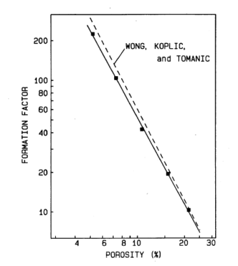
Figure 18: Log-log plot of formation factor versus porosity for sintered glass beads with 200-300 $\mu$ m diameter from [287]. The solid line is a fit to $F=a\relax\overline{\phi}^{m}$ with $a=0.33$ and cementation exponent $m=2.2$ while the dashed line represents the results $a=0.30$ and $m=2.3$ on the same system in [254]. [Reproduced with permission from I. Holwech and B. Nøst, “Dielectric dispersion measurements of salt-water saturated porous glass,” Phys.Rev.B, vol. 38, p. 12845, 1989, Copyright American Physical Society 1989.]

Note the small range of porosities in the figure. The existence of nontrivial power law relations in such samples is better demonstrated by correlating the conductivity with the permeability [284, 170]. In other experiments on artificial media a mixture of rubber balls and water is successively compressed while monitoring its conductivity [289, 217]. These experiments show deviations from the pure algebraic behaviour postulated by (5.21). If the cementation ”exponent” in (5.21) is assumed to depend on $\overline{\phi}$ then it increases at low porosities in agreement with the general trend that higher values correspond to a higher degree of compaction.

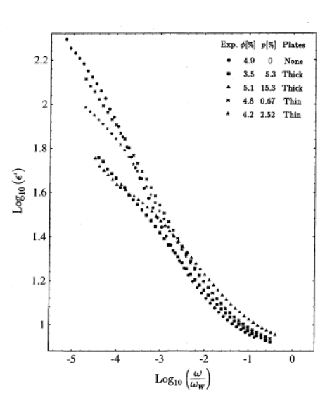
A much better confirmed observation on natural and artificial porous rocks is dielectric enhancement caused by the disorder in the microstructure [290, 291, 292, 293, 294, 287, 295, 89]. Dielectric enhancement due to disorder has been studied extensively in percolation theory and experiment [296, 297, 40]. An example is shown in figure 19 for the sintered glass bead media containing thin glass plates.

Figure 19: Log-log plot of the real part of the dielectric function versus normalized frequency $\relax\omega/\omega _{W}$ where $\relax\omega _{W}=\sigma^{{\prime}}_{W}/(\epsilon _{0}\epsilon^{{\prime}}_{W})$ is the relaxation frequency of water for samples with porosities close to 5 percent. The different symbols denote different concentrations of thin glass plates $p$ defined as the ratio of the mass of the glass plates divided by the total mass of glass in the sample [362].

In these media interfacial conductivity and other electrochemical effects can be neglected [287]. The frequency is plotted in units of $\omega _{W}=\sigma^{{\prime}}_{W}/(\epsilon _{0}\epsilon^{{\prime}}_{W})$ the relaxation frequency of water. Although salt water and glass are essentially dispersion free in the frequency range shown in figure 19 their mixture shows a pronounced dispersion which exceeds the values of the dielectric constants of both components. Similar results can be found in [287]. In [295] the dielectric response of a large number of sandstones and carbonates is given in terms of the empirical Cole-Cole formula [298]. Interestingly the corresponding temporal relaxation function appears within the recent theory of nonequilibrium systems [64] which is the same theory on which the macroscopic local porosity distributions in section III.A.5 were based.

V.B.3 Theoretical Mixing Laws

V.B.3.a Spectral Theories

Dielectric mixing laws express the frequency dependent dielectric function or conductivity of a two component mixture in terms of the dielectric functions of the constituents [46, 35, 40, 31]. Spectral theories express the effective dielectric function in terms of an abstract pole spectrum which is independent of the dielectric functions $\epsilon\rule[-4.3pt]{0.0pt}{6.45pt}_{{\mathbb{P}}}$ and $\epsilon\rule[-4.3pt]{0.0pt}{6.45pt}_{{\mathbb{M}}}$ of the two constitutents filling the pore and matrix space [299, 300, 301, 302, 303, 293, 304, 305, 306, 307, 308, 309]. Theoretically the effective dielectric function may be written as

$\overline{\epsilon}=\epsilon\rule[-4.3pt]{0.0pt}{6.45pt}_{{\mathbb{M}}}\left(1-\sum _{{n=1}}^{\infty}\frac{a_{n}}{s-b_{n}}\right)$

(5.22)

where

$s=\left(1-\frac{\epsilon\rule[-4.3pt]{0.0pt}{6.45pt}_{{\mathbb{P}}}}{\epsilon\rule[-4.3pt]{0.0pt}{6.45pt}_{{\mathbb{M}}}}\right)^{{-1}}.$

(5.23)

The constants $a_{n}$ and $b_{n}$ are the strength and location of the poles and they reflect the influence of the microgeometry. Unfortunately these parameters do not have a direct geometrical interpretation although under the assumption of stationarity and isotropy two sum rules are known which connect integrals of the pole spectrum with the bulk porosity [40].

V.B.3.b Geometric Theories

The simplest geometric theories for the effective dielectric function $\overline{\epsilon}$ are mean field theories. In these approximations a small spherical cell with a randomly valued dielectric constant $\epsilon$ is embedded into a homogeneous host medium of dielectric constant $\epsilon\rule[-4.3pt]{0.0pt}{6.45pt}_{{h}}$ . Then the electrical analogue of eq. (5.3) becomes

$\overline{\epsilon}=\epsilon\rule[-4.3pt]{0.0pt}{6.45pt}_{{h}}\left(1+2\left\langle\frac{\epsilon-\epsilon\rule[-4.3pt]{0.0pt}{6.45pt}_{{h}}}{\epsilon+2\epsilon\rule[-4.3pt]{0.0pt}{6.45pt}_{{h}}}\right\rangle\right)\left(1-\left\langle\frac{\epsilon-\epsilon\rule[-4.3pt]{0.0pt}{6.45pt}_{{h}}}{\epsilon+2\epsilon\rule[-4.3pt]{0.0pt}{6.45pt}_{{h}}}\right\rangle\right)^{{-1}}$

(5.24)

where the average denotes an ensemble average using the probability density $w(\epsilon)$ of $\epsilon$ . A two component medium $\mathbb{S}=\mathbb{P}\cup\mathbb{M}$ can be represented by the binary probability density

$w(\epsilon)=\overline{\phi}\delta(\epsilon-\epsilon\rule[-4.3pt]{0.0pt}{6.45pt}_{{\mathbb{P}}})+(1-\overline{\phi})\delta(\epsilon-\epsilon\rule[-4.3pt]{0.0pt}{6.45pt}_{{\mathbb{M}}})$

(5.25)

containing $\overline{\phi}$ as the only geometrical input parameter. The Clausius-Mossotti approximation [310, 46] for a two component medium is obtained by setting $\epsilon\rule[-4.3pt]{0.0pt}{6.45pt}_{{h}}=\epsilon\rule[-4.3pt]{0.0pt}{6.45pt}_{{\mathbb{M}}}$ in the limit $\overline{\phi}\rightarrow 1$ or $\epsilon\rule[-4.3pt]{0.0pt}{6.45pt}_{{h}}=\epsilon\rule[-4.3pt]{0.0pt}{6.45pt}_{{\mathbb{P}}}$ in the limit $\overline{\phi}\rightarrow 0$ in (5.24). In the latter case one obtains

$\frac{\overline{\epsilon}-\epsilon\rule[-4.3pt]{0.0pt}{6.45pt}_{{\mathbb{P}}}}{\overline{\epsilon}+2\epsilon\rule[-4.3pt]{0.0pt}{6.45pt}_{{\mathbb{P}}}}=(1-\overline{\phi})\frac{\epsilon\rule[-4.3pt]{0.0pt}{6.45pt}_{{\mathbb{M}}}-\epsilon\rule[-4.3pt]{0.0pt}{6.45pt}_{{\mathbb{P}}}}{\epsilon\rule[-4.3pt]{0.0pt}{6.45pt}_{{\mathbb{M}}}+2\epsilon\rule[-4.3pt]{0.0pt}{6.45pt}_{{\mathbb{P}}}}$

(5.26)

which will be a good approximation at low porosities. Note that the Clausius-Mossotti approximation is not symmetrical under exchanging pore and matrix. A symmetrical and also self consistent approximation is obtained from (5.24) by setting $\epsilon\rule[-4.3pt]{0.0pt}{6.45pt}_{{h}}=\overline{\epsilon}$ . This leads to the symmetrical effective medium approximation for a two component medium

$\overline{\phi}\frac{\epsilon\rule[-4.3pt]{0.0pt}{6.45pt}_{{\mathbb{P}}}-\overline{\epsilon}}{\epsilon\rule[-4.3pt]{0.0pt}{6.45pt}_{{\mathbb{P}}}+2\overline{\epsilon}}+(1-\overline{\phi})\frac{\epsilon\rule[-4.3pt]{0.0pt}{6.45pt}_{{\mathbb{M}}}-\overline{\epsilon}}{\epsilon\rule[-4.3pt]{0.0pt}{6.45pt}_{{\mathbb{M}}}+2\overline{\epsilon}}=0$

(5.27)

which could have been derived also from using equation (5.25) in (5.12). The effective medium approximation is a very good approximation for microstructures consisting of a small concentration of nonoverlapping spherical grains embedded in a host. Recently, much effort has been expended to show that the EMA becomes exact for certain pathological microstructures [311]. The so called asymmetrical or differential effective medium approximation is obtained by iterating the Clausius-Mossotti equation which gives the effective conductivity to lowest order in $\overline{\phi}$ [285, 312, 313]. One finds the result

(5.28)

for spherically shaped inclusions.

The symmetric and asymmetric effective medium appoximations can be generalized to ellipsoidal inclusions because the electric field and polarization inside the ellipsoid remain uniform in an applied external field [310, 40, 312]. For aligned oblate spheroids whose quadratic form is $(x/b_{2})^{2}+(y/b_{2})^{2}+(z/b_{1})^{2}=1$ with $b_{1}\leq b_{2}$ the effective medium theory for a two component composite results in two coupled equations

$\overline{\phi}\frac{\epsilon\rule[-4.3pt]{0.0pt}{6.45pt}_{{\mathbb{P}i}}-\overline{\epsilon}_{i}}{1+\Lambda _{i}(\epsilon\rule[-4.3pt]{0.0pt}{6.45pt}_{{\mathbb{P}i}}-\overline{\epsilon}_{i})}+(1-\overline{\phi})\frac{\epsilon\rule[-4.3pt]{0.0pt}{6.45pt}_{{\mathbb{M}i}}-\overline{\epsilon}_{i}}{1+\Lambda _{i}(\epsilon\rule[-4.3pt]{0.0pt}{6.45pt}_{{\mathbb{M}i}}-\overline{\epsilon}_{i})}=0$

(5.29)

where the index $i=1$ denotes vertical conductivities and the index $i=2$ horizontal conductivities. The two equations in (5.29) are coupled through

$\displaystyle\Lambda$	$\displaystyle=$	$\displaystyle\frac{L_{i}}{\overline{\epsilon}_{i}}$	(5.30)
$\displaystyle 2L_{2}$	$\displaystyle=$	$\displaystyle(-L_{1})$	(5.31)
$\displaystyle L_{1}$	$\displaystyle=$	$\displaystyle(e^{{-3}}+e^{{-1}})(e-\arctan e)$	(5.32)
$\displaystyle e$	$\displaystyle=$	$\displaystyle\sqrt{\frac{b_{2}^{2}\overline{\epsilon}_{1}}{b_{1}^{2}\overline{\epsilon}_{2}}-1}$	(5.33)

with $(1/3)\leq L_{1}\leq 1$ . The generalization of the asymmetric effective medium theory (5.28) to aligned spheroids with depolarization factor $L$ was given in [285] as

(5.34)

For spheroids with identical shape but isotropically distributed orientations

$\frac{\overline{\epsilon}-\epsilon\rule[-4.3pt]{0.0pt}{6.45pt}_{{\mathbb{M}}}}{\epsilon\rule[-4.3pt]{0.0pt}{6.45pt}_{{\mathbb{P}}}-\epsilon\rule[-4.3pt]{0.0pt}{6.45pt}_{{\mathbb{M}}}}\left(\frac{\epsilon\rule[-4.3pt]{0.0pt}{6.45pt}_{{\mathbb{P}}}}{\overline{\epsilon}}\right)^{{\frac{3L(1-L)}{1+3L}}}\left(\frac{(5-3L)\epsilon\rule[-4.3pt]{0.0pt}{6.45pt}_{{\mathbb{P}}}+(1+3L)\epsilon\rule[-4.3pt]{0.0pt}{6.45pt}_{{\mathbb{M}}}}{(5-3L)\overline{\epsilon}+(1+3L)\epsilon\rule[-4.3pt]{0.0pt}{6.45pt}_{{\mathbb{M}}}}\right)^{{\frac{2(1-3L)^{2}}{(1+3L)(5-3L)}}}=\overline{\phi}$

(5.35)

was obtained in [314, 205, 292]. Equation (5.34) will be referred to as the Sen-Scala-Cohen model (SSC) and (5.35) will be called the uniform spheroid model (USM).

Recently local porosity theory has been proposed as an alternative generalization of effective medium theories [168, 169, 170, 171, 172, 173, 174, 175]. The simplest mean field theories (5.26), (5.27) and (5.28) are based on the simplest geometric characterization theories of section III.A.1. These theories are usually interpreted geometrically in terms of grain models(see section III.B.2) with spherical grains embedded into a homogeneous host material. The generalizations (5.29), (5.34) and (5.35) are obtained by generalizing the interpretation to more general grain models. Local porosity theory on the other hand is based on generalizing the geometric characterization by using local geometry distributions (see section III.A.5) rather than simply porosity or specific surface area alone. In III.A.5 two different types of local geometry distributions were introduced: Macroscopic distributions with infinitely large measurement cells defined in (3.52), and mesoscopic distributions with measurement cells of finite volume defined in (3.33). For a mesoscopic partitioning $\mathcal{K}$ of the sample using a simple cubic lattice with cubic unit cell $\mathbb{K}$ the selfconsistency equation of local porosity theory for $\overline{\epsilon}$ reads

$\int _{0}^{1}\left[\frac{\epsilon\rule[-4.3pt]{0.0pt}{6.45pt}_{{C}}(\phi)-\overline{\epsilon}}{\epsilon\rule[-4.3pt]{0.0pt}{6.45pt}_{{C}}(\phi)+2\overline{\epsilon}}\lambda(\phi;\mathbb{K})+\frac{\epsilon\rule[-4.3pt]{0.0pt}{6.45pt}_{{B}}(\phi)-\overline{\epsilon}}{\epsilon\rule[-4.3pt]{0.0pt}{6.45pt}_{{B}}(\phi)+2\overline{\epsilon}}(1-\lambda(\phi;\mathbb{K}))\right]\mu(\phi;\mathbb{K})\; d\phi=0$

(5.36)

where $\lambda(\phi;\mathbb{K})$ is the local percolation probability defined in section III.A.5.d, and $\epsilon\rule[-4.3pt]{0.0pt}{6.45pt}_{{C}}(\phi)$ and $\epsilon\rule[-4.3pt]{0.0pt}{6.45pt}_{{B}}(\phi)$ are the local dielectric functions of percolating or conducting (index $C$ ) and nonpercolating or blocking (index $B$ ) measuremente cells. In (5.40) it is assumed that the local dielectric response depends only on the porosity, but this may be generalized to include other geometrical characteristics.

Equation (5.36) has two interesting special cases. For a cubic measurement lattice ( $z=6$ ) in the limit $L\rightarrow 0$ in which the sidelength $L$ of the cubic cells is small the one cell local porosity distribution is given by (3.31) or (3.34) if the medium is mixing. Inserting (3.31) or (3.34) into (5.36) and using $\lambda(0)=0$ , $\lambda(1)=1$ , $\epsilon\rule[-4.3pt]{0.0pt}{6.45pt}_{{C}}(0)=\epsilon\rule[-4.3pt]{0.0pt}{6.45pt}_{{B}}(0)=\epsilon\rule[-4.3pt]{0.0pt}{6.45pt}_{{\mathbb{M}}}$ and $\epsilon\rule[-4.3pt]{0.0pt}{6.45pt}_{{C}}(1)=\epsilon\rule[-4.3pt]{0.0pt}{6.45pt}_{{B}}(1)=\epsilon\rule[-4.3pt]{0.0pt}{6.45pt}_{{\mathbb{P}}}$ yields equation (5.27) for traditional effective medium theory. Note however that in the limit $L\rightarrow 0$ the local porosities become highly correlated rendering a description of the geometry in terms of the one cell function $\mu(\phi;\mathbb{K})$ more and more inadequate. This argument does not apply in the opposite limit $L\rightarrow\infty$ in which the measurement cells $\mathbb{K}$ become very large, For stationary media the local porosities in nonoverlapping measurement cells are uncorrelated in the limit $L\rightarrow\infty$ . For stationary and mixing media the local porosity distribution

$\lim _{{b\rightarrow\infty}}\mu(\phi;b\mathbb{K})=\delta(\phi-\overline{\phi})$

(5.37)

becomes concentrated at a single point according to (3.32) or (3.35). Assuming as before that the limit is independent of the shape of $\mathbb{K}$ equation (5.36) reduces to

$\lambda(\overline{\phi})\frac{\epsilon\rule[-4.3pt]{0.0pt}{6.45pt}_{{C}}(\overline{\phi})-\overline{\epsilon}}{\epsilon\rule[-4.3pt]{0.0pt}{6.45pt}_{{C}}(\overline{\phi})+2\overline{\epsilon}}+(1-\lambda(\overline{\phi}))\frac{\epsilon\rule[-4.3pt]{0.0pt}{6.45pt}_{{B}}(\overline{\phi})-\overline{\epsilon}}{\epsilon\rule[-4.3pt]{0.0pt}{6.45pt}_{{B}}(\overline{\phi})+2\overline{\epsilon}}=0$

(5.38)

which is identical to (5.27) except for the replacement of $\overline{\phi}$ by $\lambda(\overline{\phi})$ , $\epsilon\rule[-4.3pt]{0.0pt}{6.45pt}_{{\mathbb{M}}}$ by $\epsilon\rule[-4.3pt]{0.0pt}{6.45pt}_{{B}}(\overline{\phi})$ , and $\epsilon\rule[-4.3pt]{0.0pt}{6.45pt}_{{\mathbb{P}}}$ by $\epsilon\rule[-4.3pt]{0.0pt}{6.45pt}_{{C}}(\overline{\phi})$ . Repeating the same differential replacement arguments [285] that lead to (5.28) for $\lambda(\overline{\phi})$ instead of $\overline{\phi}$ gives a differential version of mesoscopic local porosity theory in the limit $L\rightarrow\infty$

$\frac{\overline{\epsilon}-\epsilon\rule[-4.3pt]{0.0pt}{6.45pt}_{{B}}(\overline{\phi})}{\epsilon\rule[-4.3pt]{0.0pt}{6.45pt}_{{C}}(\overline{\phi})-\epsilon\rule[-4.3pt]{0.0pt}{6.45pt}_{{B}}(\overline{\phi})}\left(\frac{\epsilon\rule[-4.3pt]{0.0pt}{6.45pt}_{{C}}(\overline{\phi})}{\overline{\epsilon}}\right)^{{1/3}}=\lambda(\overline{\phi}).$

(5.39)

Note that the limiting equations (5.38) and (5.39) for $L\rightarrow\infty$ contain geometric information about the pore space which goes beyond the bulk porosity, and which is contained in the function $\lambda(\overline{\phi})$ .

As discussed in section III.A.5.e the $\delta$ -distribution is not the only possible macroscopic limit. Macroscopically heterogeneous media are described by the limiting macroscopic local porosity densities $\mu(\phi;\varpi,C,D)$ defined in (3.52). The $\delta$ -distribution $\delta(\phi-\overline{\phi})$ is obtained in the limit $\varpi\rightarrow 1$ or in the degenerate case arising for $D=0$ . The macroscopic form of local porosity theory for the effective dielectric constant is given by the integral equation

$\int _{0}^{1}\left[\frac{\epsilon\rule[-4.3pt]{0.0pt}{6.45pt}_{{C}}(\phi)-\overline{\epsilon}}{\epsilon\rule[-4.3pt]{0.0pt}{6.45pt}_{{C}}(\phi)+2\overline{\epsilon}}\lambda(\phi)+\frac{\epsilon\rule[-4.3pt]{0.0pt}{6.45pt}_{{B}}(\phi)-\overline{\epsilon}}{\epsilon\rule[-4.3pt]{0.0pt}{6.45pt}_{{B}}(\phi)+2\overline{\epsilon}}(1-\lambda(\phi))\right]\mu(\phi;\varpi,C,D)\; d\phi=0$

(5.40)

with $\mu(\phi;\varpi,C,D)$ defined in (3.52) and $\varpi\neq 1$ and $D\neq 0$ . If the parameters $\varpi=\varpi(\overline{\phi},\overline{\phi^{2}},\overline{\phi^{3}})$ , $D=D(\overline{\phi},\overline{\phi^{2}},\overline{\phi^{3}})$ , and $C=C(\overline{\phi},\overline{\phi^{2}},\overline{\phi^{3}})$ , are expressed in terms of the moments according to (3.53) the resulting effective dielectric function $\overline{\epsilon}=\overline{\epsilon}(\overline{\phi},\overline{\phi^{2}},\overline{\phi^{3}})$ is found to be a function of the bulk porosity and its fluctuations. This observation indicates the possibility to study Archie’s law within the framework of local porosity theory.

V.B.4 Archies Law

Archies law (5.21) concerns the effective dc conductivity, $\sigma^{{\prime}}(0)$ , and it can be studied by replacing $\epsilon$ with $\sigma^{{\prime}}(0)$ in all the formulas of the preceding section. For notational convenience the shorthand notation $\sigma^{{\prime}}(0)=\sigma$ will be employed in this section. Archie’s law can then be discussed by replacing $\epsilon$ with $\sigma$ throughout and setting $\sigma\rule[-4.3pt]{0.0pt}{6.45pt}_{{\mathbb{M}}}=0$ . From the the Clausius-Mossotti formula (5.26) one obtains the relation

$\overline{\sigma}=\sigma\rule[-4.3pt]{0.0pt}{6.45pt}_{{\mathbb{P}}}\frac{2\overline{\phi}}{3-\overline{\phi}}$

(5.41)

which reproduces Archie’s law (5.21) with a cementation exponent $m=1$ . The symmetrical effective medium approximation (5.27) gives

$\overline{\sigma}=\frac{\sigma\rule[-4.3pt]{0.0pt}{6.45pt}_{{\mathbb{P}}}}{2}(3\overline{\phi}-1)$

(5.42)

for $\overline{\phi}>1/3$ and $\overline{\sigma}=0$ for $\overline{\phi}\leq 1/3$ . Thus the symmetrical effective medium theory predicts a percolation transition at $\overline{\phi}_{c}=1/3$ and does not agree with Archie’s law (5.21) in this respect. The same conclusion holds for the anisotropic generalization of the symmetric theory to nonspherical inclusions given in (5.29).

For the asymmetric effective medium theory in its simplest form (5.28) one finds

$\overline{\sigma}=\sigma\rule[-4.3pt]{0.0pt}{6.45pt}_{{\mathbb{P}}}\overline{\phi}^{{3/2}}$

(5.43)

consistent with Archies law (5.21) with cementation exponent $m=3/2$ . This expression has found much attention because it yields $m\neq 1$ [285, 315, 314, 205, 312]. There are, however, several problems with equation (5.43). Its derivation implies that the solid component is not connected [312]. The experimentally observed behaviour is often not algebraic, and if a power law is nevertheless assumed its exponent is often very different from $3/2$ . Most importantly, the frequency dependent theory does not predict sufficient dielectric enhancement. The first problem can be circumvented by generalizing to a three component medium [316, 313], the second can be overcome by considering nonspherical inclusions [285, 315, 314, 205, 312]. As an example the generalization to nonspherical grains (5.34) gives

$\overline{\sigma}=\sigma\rule[-4.3pt]{0.0pt}{6.45pt}_{{\mathbb{P}}}\overline{\phi}^{{1/(1-L)}}$

(5.44)

with $1/3\leq L\leq 1$ , and the uniform spheroid model gives a similar result. The most serious problem, however, is the fact pointed out in [285, 292] that (5.28) cannot reproduce the frequency dependence of $\overline{\sigma}$ and the observed dielectric enhancement. This will be discussed further in the next section.

Local porosity theory contains geometrical information above and beyond the average porosity $\overline{\phi}$ and cosequently it predicts more general relationships between porosity and conductivity. In its simplest form equation (5.38) leads to

$\overline{\sigma}=\frac{\sigma\rule[-4.3pt]{0.0pt}{6.45pt}_{{C}}(\overline{\phi})}{2}(3\lambda(\overline{\phi})-1)$

(5.45)

which may or may not have a percolation transition depending upon whether the equation

$\lambda(\overline{\phi}_{c})=\frac{1}{3}$

(5.46)

has a solution $0<\overline{\phi}_{c}<1$ which can be interpreted as a critical porosity. Therefore the percolation threshold can arise at any porosity including $\overline{\phi}_{c}=0$ , and this allows to reconcile percolation theory with Archie’s law. Note also that the behaviour is nonuniversal⁵ (This is a footnote:) ⁵ The statement in [41] that local porosity theory predicts Archies law with a universal exponent is incorrect. and depends on the local percolation probability function $\lambda(\phi)$ , and the local response $\sigma\rule[-4.3pt]{0.0pt}{6.45pt}_{{C}}(\overline{\phi})$ . Similarly the differential form (5.39) of local porosity theory yields

$\overline{\sigma}=\sigma\rule[-4.3pt]{0.0pt}{6.45pt}_{{C}}(\overline{\phi})\lambda(\overline{\phi})^{{3/2}}$

(5.47)

which is more versatile than (5.44). The preceding results hold for large measurement cells when $\mu(\phi)\approx\delta(\phi-\overline{\phi})$ . For general local porosity distributions equation (5.36) gives the result [168]

$\overline{\sigma}\approx\sigma _{0}(p-p_{c})$

(5.48)

where $p_{c}=1/3$ ,

$\frac{1}{\sigma _{0}}=\int _{0}^{1}\frac{\lambda(\phi;\mathbb{K})\mu(\phi;\mathbb{K})}{\sigma\rule[-4.3pt]{0.0pt}{6.45pt}_{{C}}(\phi)}\; d\phi,$

(5.49)

and $p$ is the control parameter of the percolation transition

$p=\int _{0}^{1}\lambda(\phi;\mathbb{K})\mu(\phi;\mathbb{K})\; d\phi$

(5.50)

giving the total fraction of percolating local geometries. The result (5.48)applies if $\overline{\phi}\rightarrow 0$ for all values of $p$ , and also if $p\rightarrow p_{c}$ at arbitrary $\overline{\phi}$ . It holds universally as long as

$\int _{0}^{1}\frac{1}{\phi}\lambda(\phi;\mathbb{K})\mu(\phi;\mathbb{K})\; d\phi<\infty$

(5.51)

the inverse first moment is finite [317]. This condition is violated for the macroscopic distributions $\mu(\phi;\varpi,C,D)$ if all cells are percolating, $\lambda(\phi)=1$ . In such a case if $\lambda(\phi)\mu(\phi)\propto\phi^{{-\alpha}}$ as $\phi\rightarrow 0$ then equation (5.48) is replaced with [317]

$\overline{\sigma}\propto(p-p_{c})^{{\frac{1}{1-\alpha(\overline{\phi},\overline{\phi^{3}},\overline{\phi^{3}})}}}$

(5.52)

where $\alpha$ depends on the moments $\overline{\phi^{n}}$ because $\varpi$ depends on them through (3.53).

Compaction and consolidation processes will in general change the local porosity distributions $\mu(\phi)$ where its dependence on $\mathbb{K}$ or the parameters $\varpi,C,D$ has been suppressed. Assume that it is possible to describe the consolidation process as a one parameter family $\mu _{q}(\phi)$ of local porosity distributions depending on a parameter $q$ which characterizes the compaction process. Then the total fraction $p$ , the bulk porosity $\overline{\phi}$ , and the integral (5.49) become functions of $q$ . If it is possible to invert the relation $\overline{\phi}=\overline{\phi}(q)$ then the fraction $p$ becomes $p=p(\overline{\phi})$ and equally $\sigma _{0}=\sigma _{0}(\overline{\phi})$ . Therefore equations (5.48) and (5.52) become porosity-conductivity relations which depend on the consolidation process.⁶ (This is a footnote:) ⁶ The statement in [41] that local porosity theory predicts Archies law with a universal cementation index is incorrect. If the condition (5.51) and the asymptotic expansions $\sigma _{0}(\overline{\phi})=\overline{\phi}^{\beta}(1+...)$ and $p(\overline{\phi})=p_{c}+\overline{\phi}^{\gamma}(p_{1}+...)$ hold then these equations yield Archies law (5.21) with a nonuniversal cementation index $m=\beta+\gamma$ . If the condition (5.51) does not hold and $\lambda(\phi)\mu(\phi)\propto\phi^{{-\alpha}}$ then

$m=\beta+\gamma\left(1+\frac{\alpha}{1-\alpha}\right)$

(5.53)

which is even less universal. The validity of the expansion $p(\overline{\phi})\propto p_{c}+\overline{\phi}^{\gamma}(p_{1}+...)$ has been tested by experiment [173, 174]. Figure 20 shows the function $p(\overline{\phi})$ obtained for sintering of glass beads.

Figure 20: Total fraction of percolating local geometries $p$ for the sintering process of $90\mu$ m glass beads as a parametrized by the bulk porosity $\overline{\phi}$ [173].

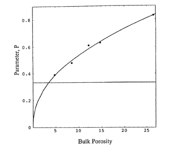
The measured data are the points, the solid curve represents a fit $p(\overline{\phi})=1.51\overline{\phi}^{{0.45}}$ through the data. This fit was chosen to indicate that the consolidation process of sintering glass beads is expected to show a percolation transition at a small but finite threshold $\overline{\phi}_{c}$ [173, 174]. Note however that the data of Figure 20 are consistent with the form $p(\overline{\phi})\propto p_{c}+\overline{\phi}(p_{1}+...)$ corresponding to $\gamma=1$ .

V.B.5 Dielectric Dispersion and Enhancement

The theoretical mixing laws for the frequency dependent dielectric function discussed in section V.B.3 can be compared with experiment. Spectral theories generally give good fits to the experimental data [293, 287] but do not allow a geometrical interpretation. Geometrical theories on the other hand contain independently observable geometric characteristics, and can be falsified by experiment.

The single parameter mean field theories (5.26), (5.12) and (5.28) contain only the bulk porosity as a geometrical quantity. They are generally unable to reproduce the observed dielectric dispersion and enhancement. This is illustrated in Figure 21 which shows the experimental measurements of the real part of the frequency dependent dielectric function as solid circles [175].

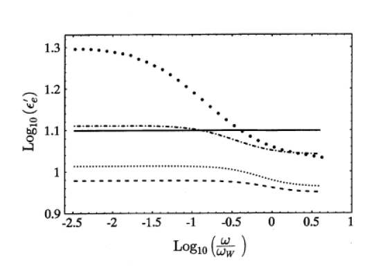
Figure 21: Comparison of simple mean field theory predictions with the experimentally observed dielectric response of sintered glass beads as a function of frequency. The solid circles are the experimental results for a $10.7\%$ sample of sintered $250\mu$ m glass beads filled with water having $\relax\sigma _{W}^{{\prime}}=12.4$ mS/m. The solid line is the Clausius-Mossotti prediction (5.26) with water background, the dashed line corresponds to the same with glass background. The dotted line is the symmetrical effective medium theory (5.27), the dash-dotted line is the asymmetrical effective medium theory (5.28) [175].

The results were obtained for a brine saturated sample of sintered $250\mu$ m glass spheres. The porosity of the specimen was $10.7\%$ , and the water conductivity was $12.4$ mS/m. A cross sectional image of the pore space has been displayed in Figure 13. The frequency in the figure is dimensionless and measured in units of the relaxation frequency of water $\omega _{W}=\sigma _{W}^{{\prime}}/(\epsilon _{0}\epsilon _{W}^{{\prime}})$ where $\sigma _{W}^{{\prime}}$ and $\epsilon _{W}^{{\prime}}$ are the conductivity and dielectric constant of water which are constant over the frequency range of interest.⁷ (This is a footnote:) ⁷ For water with $\relax\sigma _{W}^{{\prime}}=12.4$ mS/m the relaxation frequency is $\relax\omega _{W}=2.82$ MHz. With the porosity known from independent measurements the simple mean field mixing laws can be tested without adjustable parameters. The prediction of the Clausius Mossotti approximation (5.26) is shown as the solid line with water as the uniform background, and as the dashed line with glass as background. The prediction of the symmetrical effective medium theory (5.27) is shown as the dotted line. The asymmetrical (differential)effective medium scheme (5.28), shown as the dash-dotted curve, appears to reproduce the high frequency behaviour correctly, but does not give the low frequency enhancement.

To compare the experimental observations with the Sen-Scala-Cohen model (5.34) or with the uniform spheroid model (5.35) the depolarization factor $L$ of the ellipsoids has to be treated as a free fit parameter [175] In the case of local porosity theory the local porosity distributions $\mu(\phi;\mathbb{K})$ have been measured independently from cross sections through the pore space using image processing techniques. The resulting distributions have been displayed in Figure 15 for different sizes $L$ of the cubic measurement cells.⁸ (This is a footnote:) ⁸The sidelength of the measurement cell and the depolarization factor have been denoted by the same symbol $L$ . Their distinction should be clear from the context. The local percolation probability function $\lambda(\phi)$ on the other hand has not yet been measured directly from pore space reconstruction. Instead the result for $p(\overline{\phi})$ displayed as the power law fit in Figure 20 was combined with the fact that $\lambda(\overline{\phi})=p(\overline{\phi})$ in the limit of large measurement cells in which $\mu(\phi)$ becomes a $\delta$ -distribution concentrated at $\overline{\phi}$ (see eq. (3.32) or (3.35)). These observations and measurements motivate the Ansatz $\lambda(\overline{\phi})=\overline{\phi}^{\zeta}$ treating $\zeta$ as a single free fit parameter. Figure 22 shows fits for the frequency dependent real dielectric function $\overline{\epsilon}^{{\prime}}(\omega)$ and inverse formation factor $F^{{-1}}(\omega)$ . In Figure 22 the solid circles are the experimental results.

Figure 22: Log-log plot of theoretical predictions for the dielectric dispersion with experimental observations of the effect. Solid circles represent experimental measurements of the effective real dielectric constant and the effective real conductivity as a function of frequency. The dielectric function decreases from left to right, and its values are read from the labels on the left axis. The conductivity increases from left to right and is indicated o the right axis. The dotted line is obtained as a best fit to equation (5.34) with $L=0.387$ for the depolarization factor. The dashed line corresponds to the uniform spheroid model (5.34) with $L=0.597$ corresponding to an aspect ratio of $2.58$ for the oblate spheroid. The solid lines are obtained from local porosity theory (5.36) using $\zeta=0.2035$ (5.28) [175].

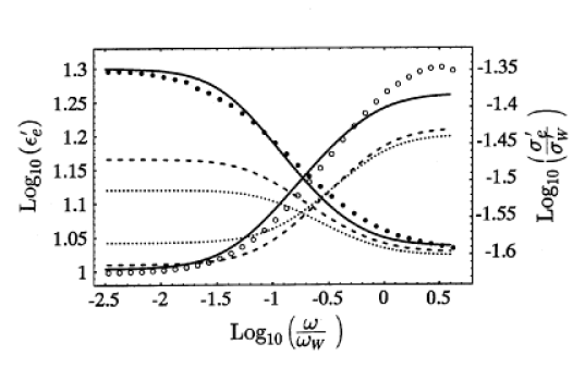
All curves represent one parameter fits to the experimental data. The solid curve is obtained from local porosity theory (5.36) using $\zeta=0.2035$ as the best value of the fit parameter. The local porosity distributions were those of Figue 15 for measurement cells of sidelength $50$ pixels. The dashed curve corresponds to the uniform spheroid model (5.35) with a depolarization factor of $0.597$ as the best value of its fit parameter. The dotted curve represents the Sen-Scala-Cohen model with a best value of $0.387$ for the depolarization.

Similar experimental results for the dielectric dispersion have been observed in natural rock samples [292]. Figure 8 in [292] compares the measurements only to the uniform spheroid model. Similar to the results of [175] on sintered glass beads the uniform spheroid model did not reproduce the dielectric enhancement, and required too high aspect ratios to be realistic for the observed microstructure.

Local porosity theory has also been used to estimate the broadening of the dielectric relaxation of polymers blends [174].

Author:	R. Hilfer
originally published in:	Advances in Chemical Physics 92, 299-424 (1996)
originally submitted:	May 9th, 1995