V.C Single Phase Fluid Flow
V.C.1 Permeability and Darcy’s Law
The permeability is the most important physical property
of a porous medium in much the same way as the porosity
is its most important geometrical property.
Some authors define porous media as media with
a nonvanishing permeability [2].
Permeability measures quantitatively the ability
of a porous medium to conduct fluid flow.
The permeability tensor ![]() relates the
macroscopic flow density
relates the
macroscopic flow density ![]() to the applied pressure
gradient
to the applied pressure
gradient ![]() or external field
or external field ![]() through
through
| (5.54) |
where ![]() is the dynamic viscosity of the fluid.
is the dynamic viscosity of the fluid.
![]() is the flow rate per unit area of cross section.
Equation (5.54) is known as Darcy’s law.
is the flow rate per unit area of cross section.
Equation (5.54) is known as Darcy’s law.
The permeability has dimensions of an area, and it is
measured in units of Darcy (d).
If the pressure is measured in physical atmospheres
one has 1d=0.9869![]() m
m![]() while 1d=1.0197
while 1d=1.0197![]() m
m![]() if the pressure is measured in technical atmospheres.
To within practical measuring accuracy one may often
assume 1d=
if the pressure is measured in technical atmospheres.
To within practical measuring accuracy one may often
assume 1d=![]() m
m![]() .
An important question arising from the fact that
.
An important question arising from the fact that ![]() is dimensionally an area concerns the interpretation of
this area or length scale in terms of the underlying geometry.
This fundamental question has recently found renewed
interest [318, 43, 319, 320, 170, 172, 4].
Unfortunately most answers proposed in these discussions
[319, 318, 320, 4]
give a dynamical rather than geometrical interpretation of
this length scale.
The traditional answer to this basic problem is provided
by hydraulic radius theory [3, 2].
It gives a geometrical interpretation which is based on the
capillary models of section III.B.1, and it will
be discussed in the next section.
is dimensionally an area concerns the interpretation of
this area or length scale in terms of the underlying geometry.
This fundamental question has recently found renewed
interest [318, 43, 319, 320, 170, 172, 4].
Unfortunately most answers proposed in these discussions
[319, 318, 320, 4]
give a dynamical rather than geometrical interpretation of
this length scale.
The traditional answer to this basic problem is provided
by hydraulic radius theory [3, 2].
It gives a geometrical interpretation which is based on the
capillary models of section III.B.1, and it will
be discussed in the next section.
The permeability does not appear in the microscopic Stokes or Navier-Stokes equations. Darcy’s law and with it the permeability concept can be derived from microscopic Stokes flow equations using homogenization techniques [268, 269, 270, 38, 321, 271] which are asymptotic expansions in the ratio of microscopic to macroscopic length scales. The derivation will be given in section V.C.3 below.
The linear Darcy law holds for flows at low Reynolds numbers in which the driving forces are small and balanced only by the viscous forces. Various nonlinear generalizations of Darcy’s law have also been derived using homogenization or volume averaging methods [268, 1, 269, 322, 321, 38, 271, 323, 324, 325]. If a nonlinear Darcy law governs the flow in a given experiment this would appear in the measurement as if the permeability becomes velocity dependent. The linear Darcy law breaks down also if the flow becomes too slow. In this case interactions between the fluid and the pore walls become important. Examples occur during the slow movement of polar liquids or electrolytes in finely porous materials with high specific internal surface.
V.C.2 Hydraulic Radius Theory
The hydraulic radius theory or Carman-Kozeny model
is based on the geometrical models of capillary
tubes discussed above in section III.B.1.
In such capillary models the permeability can be
obtained exactly from the solution of
the Navier-Stokes equation (4.9)
in the capillary.
Consider a cylindrical capillary tube of length ![]() and radius
and radius ![]() directed along the
directed along the ![]() -direction.
The velocity field
-direction.
The velocity field ![]() for creeping laminar
flow is of the form
for creeping laminar
flow is of the form ![]() where
where ![]() denotes a unit vector along the pipe, and
denotes a unit vector along the pipe, and
![]() measures the distance from the center of the pipe.
The pressure has the form
measures the distance from the center of the pipe.
The pressure has the form ![]() .
Assuming “no slip” boundary conditions,
.
Assuming “no slip” boundary conditions, ![]() , at the tube
walls one obtains for
, at the tube
walls one obtains for ![]() the familiar Hagen-Poiseuille
result [326]
the familiar Hagen-Poiseuille
result [326]
| (5.55) | ||||
| (5.56) |
with a parabolic velocity and linear pressure profile.
The volume flow rate ![]() is obtained through integration as
is obtained through integration as
| (5.57) |
Consider now the capillary tube model of section III.B.1
with a cubic sample space ![]() of sidelength
of sidelength ![]() .
The pore space
.
The pore space ![]() consists of
consists of ![]() nonintersecting capillary
tubes of radii
nonintersecting capillary
tubes of radii ![]() and lengths
and lengths ![]() distributed according
to a joint probability density
distributed according
to a joint probability density ![]() .
The pressure drop must then be calculated over the length
.
The pressure drop must then be calculated over the length ![]() and thus the right hand side of (5.57) is
multiplied by a factor
and thus the right hand side of (5.57) is
multiplied by a factor ![]() .
Because the tubes are nonintersecting the volume flow
.
Because the tubes are nonintersecting the volume flow ![]() through each of the tubes can be added to give the macroscopic
volume flow rate per unit area
through each of the tubes can be added to give the macroscopic
volume flow rate per unit area ![]() .
Thus the permeability of the capillary tube model
is simply additive, and it reads
.
Thus the permeability of the capillary tube model
is simply additive, and it reads
 |
(5.58) |
Dimensional analysis of (5.58), (3.58)
and (3.59) shows that ![]() is
dimensionless.
Averaging (5.58) as well as (3.58)
and (3.59) for the porosity and specific internal
surface of the capillary tube model yields the relation
is
dimensionless.
Averaging (5.58) as well as (3.58)
and (3.59) for the porosity and specific internal
surface of the capillary tube model yields the relation
| (5.59) |
where the mixed moment ratio
| (5.60) |
is a dimensionless number, and the angular brackets denote
as usual the average with respect to ![]() .
.
The hydraulic radius theory or
Carman-Kozeny model is obtained from a mean field
approximation which assumes ![]() .
The approximation becomes exact if the distribution is sharply
peaked or if
.
The approximation becomes exact if the distribution is sharply
peaked or if ![]() and
and ![]() for all
for all ![]() .
With this approximation
the average permeability
.
With this approximation
the average permeability ![]() may be rewritten
in terms of the average hydraulic radius
may be rewritten
in terms of the average hydraulic radius ![]() defined in
(3.66) as
defined in
(3.66) as
| (5.61) |
where ![]() is the average of the tortuosity
defined above in (3.62).
Equation (5.61) is one of the main results of
hydraulic radius theory.
The permeability is expressed as the square of an
average hydraulic radius
is the average of the tortuosity
defined above in (3.62).
Equation (5.61) is one of the main results of
hydraulic radius theory.
The permeability is expressed as the square of an
average hydraulic radius ![]() , which is related to the
average “pore width” as
, which is related to the
average “pore width” as ![]() .
.
It must be stressed that hydraulic radius theory is not exact
even for the simple capillary tube model because in general
![]() and
and ![]() .
However, interesting exact relations for the average permeability
can be obtained from (5.59) and (5.60)
in various special cases without employing the
mean field approximation of hydraulic radius theory.
If the tube radii and lengths are independent then the distribution
factorizes as
.
However, interesting exact relations for the average permeability
can be obtained from (5.59) and (5.60)
in various special cases without employing the
mean field approximation of hydraulic radius theory.
If the tube radii and lengths are independent then the distribution
factorizes as ![]() .
In this case the permeability may be written as
.
In this case the permeability may be written as
| (5.62) |
where ![]() is the average of the tortuosity factor
defined in (3.62).
The last equality interprets
is the average of the tortuosity factor
defined in (3.62).
The last equality interprets ![]() in terms of the
microscopic effective cross section
in terms of the
microscopic effective cross section ![]() determined by the variance and curtosis of the distribution
of tube radii.
Further specialization to the cases
determined by the variance and curtosis of the distribution
of tube radii.
Further specialization to the cases ![]() or
or ![]() is
readily carried out from these results.
is
readily carried out from these results.
Finally it is of interest to consider also the capillary slit
model of section III.B.1.
The model assumes again a cubic sample of side length ![]() containing a pore space consisting of parallel slits with
random widths governed by a probability density
containing a pore space consisting of parallel slits with
random widths governed by a probability density ![]() .
For flat planes without undulations the analogue of tortuosity
is absent.
The average permeability is obtained in this case as
.
For flat planes without undulations the analogue of tortuosity
is absent.
The average permeability is obtained in this case as
| (5.63) |
which has the same form as (5.59) with a constant
![]() .
The prefactor
.
The prefactor ![]() is due to the different shape of the
capillaries, which are planes rather than tubes.
is due to the different shape of the
capillaries, which are planes rather than tubes.
V.C.3 Derivation of Darcy’s Law from Stokes Equation
The previous section has shown that Darcy’s law arises in the capillary models. This raises the question whether it can be derived more generally. The present section shows that Darcy’s law can be obtained from Stokes equation for a slow flow. It arises to lowest order in an asymptotic expansion whose small parameter is the ratio of microscopic to macroscopic length scales.
Consider the stationary and creeping (low Reynolds number)
flow of a Newtonian incompressible fluid through a porous
medium whose matrix is assumed to be rigid.
The microscopic flow through the pore space ![]() is governed
by the stationary Stokes equations for the velocity
is governed
by the stationary Stokes equations for the velocity ![]() and pressure
and pressure ![]()
| (5.64) | ||||
| (5.65) |
inside the pore space, ![]() , with no slip boundary condition
, with no slip boundary condition
| (5.66) |
for ![]() .
The body force
.
The body force ![]() and the dynamic viscosity
and the dynamic viscosity ![]() are
assumed to be constant.
are
assumed to be constant.
The derivation of Darcy’s law assumes that the pore space ![]() has a characteristic length scale
has a characteristic length scale ![]() which is small compared to
some macroscopic scale
which is small compared to
some macroscopic scale ![]() .
The microscopic scale
.
The microscopic scale ![]() could be the diameter of grains,
the macroscale
could be the diameter of grains,
the macroscale ![]() could be the diameter of the sample
could be the diameter of the sample ![]() or some other macroscopic length such as the diameter of
a measurement cell or the wavelength of a seismic wave.
The small ratio
or some other macroscopic length such as the diameter of
a measurement cell or the wavelength of a seismic wave.
The small ratio ![]() provides a small parameter for
an asymptotic expansion.
The expansion is constructed by assuming that all properties
and fields can be written as functions of two new space variables
provides a small parameter for
an asymptotic expansion.
The expansion is constructed by assuming that all properties
and fields can be written as functions of two new space variables
![]() which are related to the original space variable
which are related to the original space variable
![]() as
as ![]() and
and ![]() .
All functions
.
All functions ![]() are now replaced with functions
are now replaced with functions ![]() and the slowly varying variable
and the slowly varying variable ![]() is allowed to vary
independently of the rapidly varying variable
is allowed to vary
independently of the rapidly varying variable ![]() .
This requires to replace the gradient according to
.
This requires to replace the gradient according to
| (5.67) |
and the Laplacian is replaced similarly.
The velocity and pressure are now expanded in ![]() where
the leading orders are chosen such that the solution is not
reduced to the trivial zero solution and the problem remains
physically meaningful.
In the present case this leads to the expansions [268, 280, 271]
where
the leading orders are chosen such that the solution is not
reduced to the trivial zero solution and the problem remains
physically meaningful.
In the present case this leads to the expansions [268, 280, 271]
| (5.68) | ||||
| (5.69) |
where ![]() and
and ![]() .
Inserting into (5.64), (5.65) and (5.66)
yields to lowest order in
.
Inserting into (5.64), (5.65) and (5.66)
yields to lowest order in ![]() the system of equations
the system of equations
| (5.70) | ||||
| (5.71) | ||||
| (5.72) | ||||
| (5.73) | ||||
| (5.74) |
in the fast variable ![]() .
It follows from the first equation that
.
It follows from the first equation that ![]() depends
only on the slow variable
depends
only on the slow variable ![]() , and thus it appears as an additional
external force for the determination of the dependence of
, and thus it appears as an additional
external force for the determination of the dependence of
![]() on
on ![]() from the remaining equations.
Because the equations are linear the solution
from the remaining equations.
Because the equations are linear the solution ![]() has the form
has the form
 |
(5.75) |
where the three vectors ![]() (and the scalars
(and the scalars ![]() )
are the solutions of the three systems (
)
are the solutions of the three systems (![]() )
)
| (5.76) | ||||
| (5.77) | ||||
| (5.78) |
and ![]() is a unit vector in the direction of the
is a unit vector in the direction of the
![]() -axis.
-axis.
It is now possible to average ![]() over the fast variable
over the fast variable ![]() .
The spatial average over a convex set
.
The spatial average over a convex set ![]() is defined as
is defined as
| (5.79) |
where ![]() is centered at
is centered at ![]() and
and
![]() equals
equals ![]() or
or ![]() depending
upon whether
depending
upon whether ![]() or not.
The dependence on the averaging region
or not.
The dependence on the averaging region ![]() has been indicated
explicitly.
Using the notation of (2.20) the average over all
space is obtained as the limit
has been indicated
explicitly.
Using the notation of (2.20) the average over all
space is obtained as the limit ![]() .
The function
.
The function ![]() need not to be averaged as it depends only on the slow
variable
need not to be averaged as it depends only on the slow
variable ![]() .
If
.
If ![]() is constant then
is constant then ![]() which
is known as the law of Dupuit-Forchheimer [1].
Averaging (5.75) gives Darcy’s law (5.54)
in the form
which
is known as the law of Dupuit-Forchheimer [1].
Averaging (5.75) gives Darcy’s law (5.54)
in the form
| (5.80) |
where the components ![]() of
the permeability tensor
of
the permeability tensor ![]() are expressed in terms of
the solutions
are expressed in terms of
the solutions ![]() to (5.76)–(5.78)
within the region
to (5.76)–(5.78)
within the region ![]() as
as
| (5.81) |
The permeability tensor is symmetric and positive definite
[268].
Its dependence on the configuration of the pore space ![]() and the averaging region
and the averaging region ![]() have been made explicit because
they will play an important role below.
For isotropic and strictly periodic or stationary media the
permeability tensor reduces to a constant independent of
have been made explicit because
they will play an important role below.
For isotropic and strictly periodic or stationary media the
permeability tensor reduces to a constant independent of ![]() .
For (quasi-)periodic microgeometries or (quasi-)stationary random
media averaging eq. (5.73) leads to the additional
macroscopic relation
.
For (quasi-)periodic microgeometries or (quasi-)stationary random
media averaging eq. (5.73) leads to the additional
macroscopic relation
| (5.82) |
Equations (5.80) and (5.82)
are the macroscopic laws governing the microscopic
Stokes flow obeying (5.64)–(5.66)
to leading order in ![]() .
.
The importance of the homogenization technique illustrated here in a simple example lies in the fact that it provides a systematic method to obtain the reference problem for an effective medium treatment.
Many of the examples for transport and relaxation in
porous media listed in chapter IV
can be homogenized using a similar technique [268].
The heterogeneous elliptic equation (4.2)
is of particular interest.
The linear Darcy flow derived in this section can be cast into
the form of (4.2) for the pressure field.
The permeability tensor may still depend on the slow variable ![]() ,
and it is therefore of interest to iterate the homogenization
procedure in order to see whether Darcy’s law becomes again
modified on larger scales.
This question is discussed next.
,
and it is therefore of interest to iterate the homogenization
procedure in order to see whether Darcy’s law becomes again
modified on larger scales.
This question is discussed next.
V.C.4 Iterated Homogenization
The permeability ![]() for the macroscopic Darcy flow
was obtained from homogenizing the Stokes equation by
averaging the fast variable
for the macroscopic Darcy flow
was obtained from homogenizing the Stokes equation by
averaging the fast variable ![]() over a region
over a region ![]() .
The dependence on the slow variable
.
The dependence on the slow variable ![]() allows for
macroscopic inhomogeneities of the permeability.
This raises the question whether the homogenization
may be repeated to arrive at an averaged description
for a much larger megascopic scale.
allows for
macroscopic inhomogeneities of the permeability.
This raises the question whether the homogenization
may be repeated to arrive at an averaged description
for a much larger megascopic scale.
If (5.80) is inserted into (5.82)
and ![]() is assumed the equation for the macroscopic pressure
field becomes
is assumed the equation for the macroscopic pressure
field becomes
| (5.83) |
which is identical with (4.2). The equation must be supplemented with boundary conditions which can be obtained from the requirements of mass and momentum conservation at the boundary of the region for which (5.83) was derived. If the boundary marks a transition to a region with different permeability the boundary conditions require continuity of pressure and normal component of the velocity.
Equation (5.83) holds at length scales ![]() much larger than the pore scale
much larger than the pore scale ![]() , and much larger than
diameter of the averaging region
, and much larger than
diameter of the averaging region ![]() .
To homogenize it one must therefore consider length scales
.
To homogenize it one must therefore consider length scales
![]() much larger than
much larger than ![]() such that
such that
| (5.84) |
is fulfilled.
The ratio ![]() is then a small parameter in terms of
which the homogenization procedure of the previous section can
be iterated.
The pressure is expanded in terms of
is then a small parameter in terms of
which the homogenization procedure of the previous section can
be iterated.
The pressure is expanded in terms of ![]() as
as
| (5.85) |
where now ![]() is the slow variable, and
is the slow variable, and ![]() is the rapidly varying variable.
Assuming that the medium is stationary, i.e. that
is the rapidly varying variable.
Assuming that the medium is stationary, i.e. that ![]() does not depend on the slow variable
does not depend on the slow variable ![]() ,
the result becomes [268, 280, 271]
,
the result becomes [268, 280, 271]
| (5.86) |
where ![]() is the first term in the expansion
of the pressure which is independent of
is the first term in the expansion
of the pressure which is independent of ![]() , and the
tensor
, and the
tensor ![]() has components
has components
 |
(5.87) |
given in terms of three scalar fields ![]() which
are obtained from solving an equation of the form
which
are obtained from solving an equation of the form
 |
(5.88) |
analogous to (5.76)–(5.78) in the homogenization of Stokes equation.
If the assumption of strict stationarity is relaxed the
averaged permeability depends in general on the slow variable,
and the homogenized equation (5.86) has then the
same form as the original equation (5.83).
This shows that the form of the macroscopic equation does not
change under further averaging.
This highlights the importance of the averaged permeability
as a key element of every macroscopically homogeneous description.
Note however that the averaged tensor ![]() may have a different symmetry than the original permeability.
If
may have a different symmetry than the original permeability.
If ![]() is isotropic (
is isotropic (![]() denotes
the unit matrix) then
denotes
the unit matrix) then ![]() may become anisotropic
because of the second term appearing in (5.87).
may become anisotropic
because of the second term appearing in (5.87).
V.C.5 Network Model
Consider a porous medium described by equation
(5.83) for Darcy flow with a stationary
and isotropic local permeability function
![]() .
The expressions (5.87) and (5.88) for the
the effective permeability tensor
.
The expressions (5.87) and (5.88) for the
the effective permeability tensor ![]() are difficult to
use for general random microstructures.
Therefore it remains necessary
to follow the strategy outlined in section V.A.2
and to discretize (5.83) using a finite difference
scheme with lattice constant
are difficult to
use for general random microstructures.
Therefore it remains necessary
to follow the strategy outlined in section V.A.2
and to discretize (5.83) using a finite difference
scheme with lattice constant ![]() .
As before it is assumed that
.
As before it is assumed that ![]() where
where ![]() is
the pore scale and
is
the pore scale and ![]() is the system size.
The discretization results in the linear network equations (5.5)
for a regular lattice with lattice constant
is the system size.
The discretization results in the linear network equations (5.5)
for a regular lattice with lattice constant ![]() .
.
To make further progress it is necessary to specify the local permeabilities. A microscopic network model of tubes results from choosing the expression
| (5.89) |
for a cylindrical capillary tube of radius ![]() and length
and length ![]() in a region of size
in a region of size ![]() .
The parameters
.
The parameters ![]() and
and ![]() must obey the geometrical
conditions
must obey the geometrical
conditions ![]() and
and ![]() .
In the resulting network model each bond
represents a winding tube with circular cross
section whose diameter and length fluctuate
from bond to bond.
The network model is completely specified by assuming
that the local geometries specified by
.
In the resulting network model each bond
represents a winding tube with circular cross
section whose diameter and length fluctuate
from bond to bond.
The network model is completely specified by assuming
that the local geometries specified by ![]() and
and ![]() are independent and identically distributed random
variables with joint probability density
are independent and identically distributed random
variables with joint probability density ![]() .
Note that the probability density
.
Note that the probability density ![]() depends
also on the discretization length through the constraints
depends
also on the discretization length through the constraints
![]() and
and ![]() .
.
Using the effective medium approximation to the network
equations the effective permeability ![]() for this
network model is the solution of the selfconsistency equation
for this
network model is the solution of the selfconsistency equation
| (5.90) |
where the restrictions on ![]() and
and ![]() are reflected
in the limits of integration.
In simple cases, as for binary or uniform distributions,
this equation can be solved analytically, in other
cases it is solved numerically.
The effective medium prediction agrees well with
an exact solution of the network equations
[231].
The behaviour of the effective permeability depends
qualitatively on the fraction
are reflected
in the limits of integration.
In simple cases, as for binary or uniform distributions,
this equation can be solved analytically, in other
cases it is solved numerically.
The effective medium prediction agrees well with
an exact solution of the network equations
[231].
The behaviour of the effective permeability depends
qualitatively on the fraction ![]() of conducting tubes
defined as
of conducting tubes
defined as
| (5.91) |
where ![]() .
For
.
For ![]() the permeability is positive while
for
the permeability is positive while
for ![]() it vanishes.
At
it vanishes.
At ![]() the network has a percolation transition.
Note that
the network has a percolation transition.
Note that ![]() is not related to the
average porosity.
is not related to the
average porosity.
V.C.6 Local Porosity Theory
Consider, as in the previous section, a porous medium described
by equation (5.83) for Darcy flow with a stationary
and isotropic local permeability function ![]() .
A glance at section III shows that the one cell
local geometry distribution defined in (3.45) are particularly
well adapted to the discretization of (5.83).
As before the discretization employs a cubic lattice with lattice
constant
.
A glance at section III shows that the one cell
local geometry distribution defined in (3.45) are particularly
well adapted to the discretization of (5.83).
As before the discretization employs a cubic lattice with lattice
constant ![]() and cubic measurement cells
and cubic measurement cells ![]() and yields a
local geometry distribution
and yields a
local geometry distribution ![]() .
It is then natural to use the Carman equation (5.59)
locally because it is often an accurate description
as illustrated in Figure 23.
.
It is then natural to use the Carman equation (5.59)
locally because it is often an accurate description
as illustrated in Figure 23.
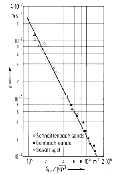
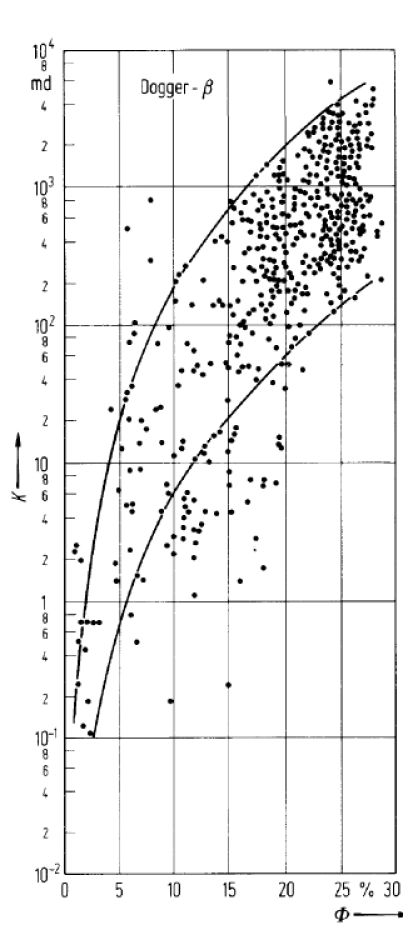
The straight line in Figure 23 corresponds to equation (5.59). The local percolation probabilities defined in section III.A.5.d complete the description. Each local geometry is characterized by its local porosity, specific internal surface and a binary random variable indicating whether the geometry is percolating or not. The selfconsistent effective medium equation now reads
| (5.92) |
for the effective permeability ![]() .
The control parameter for the underlying percolation transition
was given in (3.47) as
.
The control parameter for the underlying percolation transition
was given in (3.47) as
| (5.93) |
and it gives the total fraction of percolating local geometries. If the quantity
 |
(5.94) |
is finite then the solution to (5.92) is given approximately as
| (5.95) |
for ![]() and as
and as ![]() for
for ![]() .
This result is analogous to (5.48) for the
electrical conductivity.
Note that the control parameter for the underlying percolation
transition differs from the bulk porosity
.
This result is analogous to (5.48) for the
electrical conductivity.
Note that the control parameter for the underlying percolation
transition differs from the bulk porosity ![]() .
.
To study the implications of (5.92) it is necessary
to supply explicit expressions for the local geometry distribution
![]() .
Such an expression is provided by the local porosity reduction
model reviewed in section III.B.6.
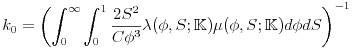
Writing the effective medium approximation for the number
.
Such an expression is provided by the local porosity reduction
model reviewed in section III.B.6.
Writing the effective medium approximation for the number ![]() defined in (3.87) and using equations (3.86)
and (3.88) it has been shown that the effective
permeability may be written approximately as [170]
defined in (3.87) and using equations (3.86)
and (3.88) it has been shown that the effective
permeability may be written approximately as [170]
| (5.96) |
where the exponent ![]() depends on the porosity reduction
factor
depends on the porosity reduction
factor ![]() and the type of consolidation model characterized by
(3.88) as
and the type of consolidation model characterized by
(3.88) as
| (5.97) |
If all local geometries are percolating, i.e. if ![]() ,
then the effective permeability depends algebraically on the
bulk porosity
,
then the effective permeability depends algebraically on the
bulk porosity ![]() with a strongly nonuniversal
exponent
with a strongly nonuniversal
exponent ![]() .
This dependence will be modified if the local percolation
probability
.
This dependence will be modified if the local percolation
probability![]() is not constant.
The large variability is consistent with experience from
measuring permeabilities in experiment.
Figure 24 demonstrates the large data scatter
seen in experimental results.
While in general small permeabilities correlate with small
porosities the correlation is not very pronounced.
is not constant.
The large variability is consistent with experience from
measuring permeabilities in experiment.
Figure 24 demonstrates the large data scatter
seen in experimental results.
While in general small permeabilities correlate with small
porosities the correlation is not very pronounced.