VI.C Macroscopic Description
VI.C.1 Macroscopic Equations of Motion
The accepted large scale equations of motion for two phase flow involve a generalization of Darcy’s law to relative permeabilities including offdiagonal viscous coupling terms [349, 270, 322, 321, 350, 351, 352]. The importance of viscous coupling terms has been recognized relatively late [353, 354, 355, 356, 357]. The equations which are generally believed to describe multiphase flow on the reservoir scale as well as on the laboratory scale may be written as [322, 350]
![\begin{array}[]{rcl}\overline{\phi}\frac{\displaystyle\partial\overline{S}_{{\scriptscriptstyle{\mathbb{W}}}}}{\displaystyle\partial\overline{t}}&=&\overline{\mbox{\boldmath$\nabla$}}\cdot\overline{\bf v}_{{\scriptscriptstyle{\mathbb{W}}}}\\
\overline{\phi}\frac{\displaystyle\partial\overline{S}_{{\scriptscriptstyle{\mathbb{O}}}}}{\displaystyle\partial\overline{t}}&=&\overline{\mbox{\boldmath$\nabla$}}\cdot\overline{\bf v}_{{\scriptscriptstyle{\mathbb{O}}}}\end{array}](mi/mi1182.png) |
(6.38) |
![\begin{array}[]{rcl}\overline{\bf v}_{{\scriptscriptstyle{\mathbb{W}}}}&=&-\left[{\bf K}^{r}_{{{\scriptscriptstyle{\mathbb{W}}}{\scriptscriptstyle{\mathbb{W}}}}}\:\frac{\displaystyle{\bf K}}{\displaystyle\mu _{{\scriptscriptstyle{\mathbb{W}}}}}\:(\overline{\mbox{\boldmath$\nabla$}}\overline{P}_{{\scriptscriptstyle{\mathbb{W}}}}-\rho _{{\scriptscriptstyle{\mathbb{W}}}}g\:\overline{\mbox{\boldmath$\nabla$}}\overline{z})+{\bf K}^{r}_{{{\scriptscriptstyle{\mathbb{W}}}{\scriptscriptstyle{\mathbb{O}}}}}\:\frac{\displaystyle{\bf K}}{\displaystyle\mu _{{\scriptscriptstyle{\mathbb{O}}}}}\:(\overline{\mbox{\boldmath$\nabla$}}\overline{P}_{{\scriptscriptstyle{\mathbb{O}}}}-\rho _{{\scriptscriptstyle{\mathbb{O}}}}g\:\overline{\mbox{\boldmath$\nabla$}}\overline{z})\right]\\
\overline{\bf v}_{{\scriptscriptstyle{\mathbb{O}}}}&=&-\left[{\bf K}^{r}_{{{\scriptscriptstyle{\mathbb{O}}}{\scriptscriptstyle{\mathbb{W}}}}}\:\frac{\displaystyle{\bf K}}{\displaystyle\mu _{{\scriptscriptstyle{\mathbb{W}}}}}\:(\overline{\mbox{\boldmath$\nabla$}}\overline{P}_{{\scriptscriptstyle{\mathbb{W}}}}-\rho _{{\scriptscriptstyle{\mathbb{W}}}}g\:\overline{\mbox{\boldmath$\nabla$}}\overline{z})+{\bf K}^{r}_{{{\scriptscriptstyle{\mathbb{O}}}{\scriptscriptstyle{\mathbb{O}}}}}\:\frac{\displaystyle{\bf K}}{\displaystyle\mu _{{\scriptscriptstyle{\mathbb{O}}}}}\:(\overline{\mbox{\boldmath$\nabla$}}\overline{P}_{{\scriptscriptstyle{\mathbb{O}}}}-\rho _{{\scriptscriptstyle{\mathbb{O}}}}g\:\overline{\mbox{\boldmath$\nabla$}}\overline{z})\right]\end{array}](mi/mi1181.png) |
(6.39) |
| (6.40) |
| (6.41) |
where ![]() denotes the macroscopic volume averaged equivalent of the
pore scale quantity
denotes the macroscopic volume averaged equivalent of the
pore scale quantity ![]() . In the equations above
. In the equations above ![]() stands for the
absolute (single phase flow) permeability tensor,
stands for the
absolute (single phase flow) permeability tensor, ![]() is the relative permeability tensor for water,
is the relative permeability tensor for water, ![]() the
oil relative permeability tensor, and
the
oil relative permeability tensor, and ![]() denote the possibly anisotropic coupling terms. The relative
permeabilities are matrix valued functions of saturation.
The saturations are denoted as
denote the possibly anisotropic coupling terms. The relative
permeabilities are matrix valued functions of saturation.
The saturations are denoted as ![]() and they
depend on the macroscopic space and time variables
and they
depend on the macroscopic space and time variables ![]() .
The capillary pressure curve
.
The capillary pressure curve ![]() and the relative
permeability tensors
and the relative
permeability tensors ![]() must be
known either from solving the pore scale equations of motion,
or from experiment.
must be
known either from solving the pore scale equations of motion,
or from experiment.
![]() and
and ![]() are conventionally
assumed to be independent of
are conventionally
assumed to be independent of ![]() and
and ![]() and this convention
is followed here, although it is conceivable that this is not
generally correct [354].
and this convention
is followed here, although it is conceivable that this is not
generally correct [354].
Eliminating ![]() and choosing
and choosing ![]() and
and ![]() as the principal unknowns one arrives at the large scale two-phase flow
equations
as the principal unknowns one arrives at the large scale two-phase flow
equations
| (6.42) | ||||
| (6.43) | ||||
for these two unknowns. Equations (6.42) and (6.43) are coupled nonlinear partial differential equations for the large scale pressure and saturation field of the water phase.
These equations must be complemented with large scale boundary conditions. For core experiments these are typically given by a surface source on one side of the core, a surface sink on the opposite face, and impermeable walls on the other faces. For a reservoir the boundary conditions depend upon the drive configuration and the geological modeling of the reservoir environment, so that Dirichlet as well as von Neumann problems arise in practice [339, 351, 352].
VI.C.2 Macroscopic Dimensional Analysis
The large scale equations of motion can be cast in dimensionless form using the definitions
| (6.44) |
 |
(6.45) |
| (6.46) |
 |
(6.47) |
| (6.48) |
where as before ![]() denotes the dimensionless
equivalent of the macroscopic quantity
denotes the dimensionless
equivalent of the macroscopic quantity ![]() . The length
. The length
![]() is now a macroscopic length,
and
is now a macroscopic length,
and ![]() a macroscopic (seepage or Darcy) velocity. The pressure
a macroscopic (seepage or Darcy) velocity. The pressure
![]() denotes the “breakthrough” pressure from the capillary
pressure curve
denotes the “breakthrough” pressure from the capillary
pressure curve ![]() . It is defined as
. It is defined as
| (6.49) |
where ![]() is the breakthrough saturation defined as the solution
of the equation
is the breakthrough saturation defined as the solution
of the equation
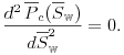 |
(6.50) |
Thus the dimensionless pressure is defined in terms of the inflection
point ![]() on the capillary pressure curve, and it gives a
measure of the macroscopic capillary pressure. Note that
on the capillary pressure curve, and it gives a
measure of the macroscopic capillary pressure. Note that ![]() is
process dependent, i.e. it will in general differ between imbibition
and drainage. This dependence reflects the influence of microscopic
wetting properties [348] and flow mechanisms on the macroscale
[358].
is
process dependent, i.e. it will in general differ between imbibition
and drainage. This dependence reflects the influence of microscopic
wetting properties [348] and flow mechanisms on the macroscale
[358].
The definition (6.48) differs from the traditional analysis [49, 329, 330, 331]. In the traditional analysis the normalized pressure field is defined as
| (6.51) |
which immediately gives rise to three problems. Firstly the permeablity is a tensor, and thus a certain nonuniqueness results in anisotropic situations [339]. Secondly equation (6.51) neglects the importance of microscopic wetting and saturation history dependence. The main problem however is that Eq. (6.51) is not based on macroscopic capillary pressures but on Darcy’s law which describes macroscopic viscous pressure effects. On the other hand the normalization (6.48) is free from these problems and it includes macroscopic capillarity in the same way as the microscopic normalization (6.15) includes microscopic capillarity.
With the normalizations introduced above the dimensionless form of the macroscopic two-phase flow equations (6.42),(6.43) becomes
| (6.52) | ||||
| (6.53) | ||||
In these equations the dimensionless tensor
| (6.54) |
plays the role of a macroscopic or large scale capillary number. Similarly the tensor
| (6.55) |
corresponds to the macroscopic gravity number.
If the traditional normalization (6.51) is used instead of the normalization (6.48), and isotropy is assumed then the same dimensionless equations are obtained with
| (6.56) |
where ![]() is the macroscopic capillary number. Thus the
traditional normalization is equivalent to the assumption that
the macroscopic viscous pressure drop always equals the
macroscopic capillary pressure. While this assumption is
not generally valid, it sometimes is a reasonable approximation
as will be illustrated below. First, however, the consequences
of the traditional assumption (6.56) for the measurement of
relative permeabilities will be discussed.
is the macroscopic capillary number. Thus the
traditional normalization is equivalent to the assumption that
the macroscopic viscous pressure drop always equals the
macroscopic capillary pressure. While this assumption is
not generally valid, it sometimes is a reasonable approximation
as will be illustrated below. First, however, the consequences
of the traditional assumption (6.56) for the measurement of
relative permeabilities will be discussed.
VI.C.3 Measurement of Relative Permeabilities
For simplicity only the isotropic case will be considered from
now on, i.e. let ![]() where
where ![]() is the
identity matrix. The tensors
is the
identity matrix. The tensors ![]() and
and ![]() then
become
then
become ![]() and
and ![]() where
where ![]() and
and ![]() are the macroscopic capillary and
gravity numbers.
are the macroscopic capillary and
gravity numbers.
The unsteady state or displacement method of measuring relative permeabilities consists of monitoring the production history and pressure drop across the sample during a laboratory displacement process [2, 359, 337]. The relative permeability is obtained as the solution of an inverse problem. The inverse problem consists in matching the measured production history and pressure drop to the solutions of the multiphase flow equations (6.52) and (6.53) using the Buckley-Leverett approximation.
In the present formulation the Buckley-Leverett approximation comprises several independent assumptions. Firstly it is assumed that gravity effects are absent, which amounts to the assumption
| (6.57) |
Secondly the viscous coupling terms are neglected, i.e.
| (6.58) |
Finally the resulting equations
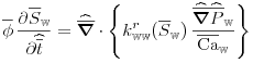 |
(6.59) |
![\overline{\phi}\,\frac{\displaystyle\partial(1-\overline{S}_{{\scriptscriptstyle{\mathbb{W}}}})}{\displaystyle\partial\widehat{\overline{t}}}=\widehat{\overline{\mbox{\boldmath$\nabla$}}}\cdot\left\{ k^{r}_{{{\scriptscriptstyle{\mathbb{O}}}{\scriptscriptstyle{\mathbb{O}}}}}(\overline{S}_{{\scriptscriptstyle{\mathbb{W}}}})\,\frac{\displaystyle\mu _{{\scriptscriptstyle{\mathbb{W}}}}}{\displaystyle\mu _{{\scriptscriptstyle{\mathbb{O}}}}}\:\left[\frac{\widehat{\overline{\mbox{\boldmath$\nabla$}}}\widehat{\overline{P}}_{{\scriptscriptstyle{\mathbb{W}}}}}{\overline{\rm Ca}_{{\scriptscriptstyle{\mathbb{W}}}}}+\frac{\widehat{\overline{\mbox{\boldmath$\nabla$}}}\widehat{\overline{P}}_{c}(\overline{S}_{{\scriptscriptstyle{\mathbb{W}}}})}{\overline{\rm Ca}_{{\scriptscriptstyle{\mathbb{W}}}}}\right]\right\}.](mi/mi1195.png) |
(6.60) |
are further simplified by assuming that the term involving
![]() in equation (6.60) may be neglected
[332].
in equation (6.60) may be neglected
[332].
Combining (6.57) with the traditional normalization (6.56) yields the consistency condition
| (6.61) |
for the application of Buckley-Leverett theory in the determination
of relative permeabilities. It is now clear from the definition
of the macroscopic gravity number, see Eq. (6.55), that
the consistent use of Buckley-Leverett theory for the unsteady
state measurement of relative permeabilities depends strongly on
the flow regime. This is valid whether or not the capillary pressure
term ![]() in (6.60) is neglected.
In addition to these consistency problems the Buckley-Leverett
theory is also plagued with stability problems [360].
in (6.60) is neglected.
In addition to these consistency problems the Buckley-Leverett
theory is also plagued with stability problems [360].
VI.C.4 Pore Scale to Large Scale Comparison
The comparison between the macroscopic and the microscopic dimensional analysis is carried out by relating the microscopic and macroscopic velocities and length scales. The macroscopic velocity is taken to be a Darcy velocity defined as (see discussion following equation (5.79))
| (6.62) |
where ![]() is the bulk porosity and
is the bulk porosity and ![]() denotes the average
microscopic flow velocity introduced in the microscopic analysis
(Eq. (6.12)). The length scales
denotes the average
microscopic flow velocity introduced in the microscopic analysis
(Eq. (6.12)). The length scales ![]() and
and ![]() are identical (
are identical (![]() ).
).
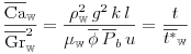
Using these relations between microscopic and macroscopic length and time scales together with the assumption of isotropy yields
| (6.63) |
as the relationship between microscopic and macroscopic capillary numbers. Similarly one obtains
| (6.64) |
for the gravity numbers. Taking the quotient gives
| (6.65) |
for the macroscopic gravillary number. Note that the ratio
![]() is the ratio of the microscopic to the macroscopic capillary
pressures. The characteristic numbers
is the ratio of the microscopic to the macroscopic capillary
pressures. The characteristic numbers
| (6.66) | ||||
| (6.67) | ||||
| (6.68) |
are the macroscopic counterparts of the microscopic numbers defined in equations (6.22), (6.30) and (6.34).
An interesting way of rewriting these relationships arises from
interpreting the permeability as an effective microscopic
cross sectional area of flow, combined with the Leverett ![]() -function.
More precisely, let
-function.
More precisely, let
 |
(6.69) |
denote a microscopic length which is characteristic for the pore space transport properties. Then equations (6.63), (6.64) and (6.65) may be rewritten as
| (6.70) | ||||
 |
(6.71) | |||
| (6.72) |
where ![]() is the value of the Leverett-
is the value of the Leverett-![]() -function [28, 2] at
the saturation corresponding to breakthrough, and
-function [28, 2] at
the saturation corresponding to breakthrough, and ![]() is the
wetting angle.
is the
wetting angle.
VI.C.5 Macroscopic Estimates
The present section gives order of magnitude estimates for the relative importance of capillary, viscous and gravity effects at different scales in representative categories of porous media. These estimates illustrate the usefulness of the macroscopic dimensionless ratios for the problem of upscaling.
Three types of porous media are considered: high permeability
unconsolidated sand, intermediate permeability sandstone
and low permeability limestone. Representative values for
![]() and
and ![]() are shown in Table VI.
are shown in Table VI.
| Quantity | Sand | Sandstone | Limestone |
|---|---|---|---|
| 0.36 | 0.22 | 0.20 | |
| 10000 mD | 400 mD | 3 mD | |
| 2000 Pa |
|
|
| Quantity | Definition | Unconsolidated Sand | Sandstone | Limestone | |||
|---|---|---|---|---|---|---|---|
| Laboratory | Reservoir | Laboratory | Reservoir | Laboratory | Reservoir | ||
|
|
|||||||
|
|
|||||||
|
|
|||||||
|
|
|||||||
|
|
|||||||
|
|
|||||||
To estimate the dimensionless numbers the same microscopic velocity
![]() as for the
microscopic estimates will be used. The length scale
as for the
microscopic estimates will be used. The length scale ![]() , however,
differs between a laboratory displacement and a reservoir process.
, however,
differs between a laboratory displacement and a reservoir process.
![]() and
and ![]() are used as representative values.
Combining these values with those in Table IV and VI
yields the results shown in Table VII.
are used as representative values.
Combining these values with those in Table IV and VI
yields the results shown in Table VII.
The first row in Table VII can be used to check the consistency of the Buckley-Leverett approximation with the traditional normalization. The consistency condition (Eq. (6.61)) is violated for unconsolidated sand and sandstones. Such a conclusion, of course, assumes that the values given in Table VI are representative for these media.
The fifth row in Table VII gives the ratio between macroscopic
and microscopic capillary numbers which according to Eq. (6.63)
is length scale dependent. The last row in Table VII compares this
ratio to the typical critical capillary number ![]() reported for
laboratory desaturation curves in the different porous media.
Using the
reported for
laboratory desaturation curves in the different porous media.
Using the ![]() for sand,
for sand,
![]() for sandstone, and
for sandstone, and
![]() for limestone [28]
as before one finds that the corresponding critical macroscopic
capillary number is close to 1.
This indicates that the macroscopic capillary number is indeed
an appropriate measure of the relative strength of viscous and
capillary forces.
for limestone [28]
as before one finds that the corresponding critical macroscopic
capillary number is close to 1.
This indicates that the macroscopic capillary number is indeed
an appropriate measure of the relative strength of viscous and
capillary forces.
As a consequence one expects differences between residual oil saturation
![]() in laboratory and reservoir floods. Given a laboratory
measured capillary desaturation curve
in laboratory and reservoir floods. Given a laboratory
measured capillary desaturation curve ![]() as a function
of the microscopic capillary number
as a function
of the microscopic capillary number ![]() the analysis predicts
that the residual oil saturation in a reservoir flood can be estimated
from the laboratory curve as
the analysis predicts
that the residual oil saturation in a reservoir flood can be estimated
from the laboratory curve as ![]() [47, 48].
For
[47, 48].
For ![]() the
the ![]() value based on macroscopic capillary
numbers will in general be lower than the value
value based on macroscopic capillary
numbers will in general be lower than the value ![]() expected from using microscopic capillary numbers. Such differences have
been frequently observed, and Morrow [361] has recently raised the
question why field recoveries are sometimes significantly higher than
those observed in the laboratory. The revised macroscopic analysis of
[47, 48] suggests a possible answer to this question.
expected from using microscopic capillary numbers. Such differences have
been frequently observed, and Morrow [361] has recently raised the
question why field recoveries are sometimes significantly higher than
those observed in the laboratory. The revised macroscopic analysis of
[47, 48] suggests a possible answer to this question.
The values of the dimensionless numbers in Table VII allow an assessment
of the relative importance of the different forces for a displacement.
To illustrate this consider the values ![]() ,
, ![]() and
and ![]() for unconsolidated sand on the laboratory scale.
A moments reflection shows that this implies
for unconsolidated sand on the laboratory scale.
A moments reflection shows that this implies ![]() where
where ![]() stands for macroscopic viscous forces,
stands for macroscopic viscous forces, ![]() for macroscopic
capillary forces, and
for macroscopic
capillary forces, and ![]() for gravity forces. The notation
for gravity forces. The notation ![]() indicates that
indicates that ![]() while
while ![]() means
means ![]() and
and ![]() stands for
stands for ![]() .
Repeating this for all cases in Table VII yields the results shown in
Table VIII. Table VIII contains also the results from the microscopic
dimensional analysis, as well as the results one would obtain from a
traditional macroscopic dimensional analysis which assumes
.
Repeating this for all cases in Table VII yields the results shown in
Table VIII. Table VIII contains also the results from the microscopic
dimensional analysis, as well as the results one would obtain from a
traditional macroscopic dimensional analysis which assumes ![]() (see Eq.
(6.56)).
(see Eq.
(6.56)).
| Sand | Sandstone | Limestone | |||
|---|---|---|---|---|---|
| pore scale |
|
||||
| traditional analysis |
|
||||
| large scale | [47] | laboratory scale |
|
||
| [48] | field scale |
|
|||
Obviously, the relative importance of the different forces may change depending on the type of medium, the characteristic fluid velocities and the length scale. Perhaps this explains part of the general difficulty of scaling up from the laboratory to the reservoir scale for immiscible displacement.
VI.C.6 Applications
The characteristic macroscopic velocities, length scales and kinematic viscosities defined respectively in equations (6.66), (6.67) and (6.68) are intrinsic physical characteristics of the porous media and the fluid displacement processes. These characteristics can be useful in applications such as estimating the width of a gravitational segregation front, the energy input required to mobilize residual oil or gravitational relaxation times.
The macroscopic gravillary number ![]() defines an intrinsic
length scale
defines an intrinsic
length scale ![]() (see Eq. (6.65)). Because
(see Eq. (6.65)). Because ![]() gives the ratio of the
gravity to the capillary forces the length
gives the ratio of the
gravity to the capillary forces the length ![]() directly
gives the width of a gravitational segregation front when the
fluids are at rest and in gravitational equilibrium, i.e. when
viscous forces are negligible or absent. Using the same estimates
for
directly
gives the width of a gravitational segregation front when the
fluids are at rest and in gravitational equilibrium, i.e. when
viscous forces are negligible or absent. Using the same estimates
for ![]() and
and ![]() as those used for Table VII one obtains
a characteristic front width of
as those used for Table VII one obtains
a characteristic front width of ![]() cm for unconsolidated sand,
cm for unconsolidated sand,
![]() m for sandstone, and roughly
m for sandstone, and roughly ![]() m for a low permeability
limestone.
m for a low permeability
limestone.
Similarly, the macroscopic capillary number defines an intrinsic
specific action (or energy input) ![]() via Eq. (6.63)
which is the energy input required to mobilize residual oil if
gravity forces may be considered negligible or absent. Represenative
estimates are given in Table IX below.
via Eq. (6.63)
which is the energy input required to mobilize residual oil if
gravity forces may be considered negligible or absent. Represenative
estimates are given in Table IX below.
The gravitational relaxation time is the time needed to return to gravitational equilibrium after its disturbance. This may be defined from the balance of gravitational forces versus the combined effect of viscous and capillary forces. Analogous to equation (6.35) for the microscopic case the dimensionless ratio becomes
| (6.73) | ||||
 |
which defines the gravitational relaxation time ![]() as
as
| (6.74) |
Estimated values are given in Table IX. They correspond to gravitational
relaxation times of roughly
![]() minutes for unconsolidated sand,
minutes for unconsolidated sand, ![]() hours for a sandstone
and
hours for a sandstone
and ![]() days for a low permeability limestone.
days for a low permeability limestone.
Another interesting intrinsic number arises from comparing the strength of macroscopic capillary forces versus the combined effect of viscous and gravity forces
| (6.75) | ||||
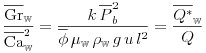 |
where ![]() denotes the volumetric flow rate. Thus
denotes the volumetric flow rate. Thus ![]() defined as
defined as
 |
(6.76) |
is an intrinsic system specific characteristic flow rate.
The estimates for ![]() and
and ![]() are summarized in Table IX.
are summarized in Table IX.
| Quantity | Sand | Sandstone | Limestone |
|---|---|---|---|
|
|
|||
|
|
|||
|
|
|||
|
|
|
||
|
|
In summary, the dimensional analysis of the upscaling problem
for two phase immiscible displacement suggests to normalize the
macroscopic pressure field in a way which differs from the
traditional normalization.
This gives rise to a macroscopic capillary number ![]() which
differs from the traditional microscopic capillary number
which
differs from the traditional microscopic capillary number ![]() in that it depends on length scale and the breakthrough capillary
pressure
in that it depends on length scale and the breakthrough capillary
pressure ![]() .
The traditional normalization corresponds to the tacit
assumption that viscous and capillary forces are of equal magnitude.
With the new macroscopic capillary number
.
The traditional normalization corresponds to the tacit
assumption that viscous and capillary forces are of equal magnitude.
With the new macroscopic capillary number ![]() the breakpoint
the breakpoint
![]() in capillary desaturation curves seems to occur
at
in capillary desaturation curves seems to occur
at ![]() for all types of porous media.
Representative estimates of
for all types of porous media.
Representative estimates of ![]() for unconsolidated sand, sandstones
and limestones suggest that the residual oil saturation after a field
flood will in general differ from that after a laboratory flood performed
under the same conditions.
Order of magnitude estimates of gravitational relaxation times and
segregation front widths for different media are consistent with
experiment.
for unconsolidated sand, sandstones
and limestones suggest that the residual oil saturation after a field
flood will in general differ from that after a laboratory flood performed
under the same conditions.
Order of magnitude estimates of gravitational relaxation times and
segregation front widths for different media are consistent with
experiment.
