2 Method of Calculation
[page 639, §1]
2.1 Recursion Relation
[639.1.1] In the rest of this paper ![]() and
and ![]() are real numbers with
are real numbers with ![]() .
[639.1.2] Calculating
.
[639.1.2] Calculating ![]() for the case
for the case ![]() can
be reduced to the case
can
be reduced to the case ![]() by virtue
of the recursion relation [2, 21]
by virtue
of the recursion relation [2, 21]
| (6) |
valid for all ![]() ,
, ![]() where
where
![]() .
[639.1.3] Here
.
[639.1.3] Here ![]() denotes the largest integer smaller than
denotes the largest integer smaller than ![]() .
[639.1.4] Because of the recursion we consider
only the case
.
[639.1.4] Because of the recursion we consider
only the case ![]() in the following.
in the following.
2.2 Regions
[639.2.1] For ![]() the complex
the complex ![]() -plane is partitioned into four
regions
-plane is partitioned into four
regions ![]() ,
, ![]() ,
, ![]() ,
, ![]() .
[639.2.2] In each region a different method
is used for the calculation of the Mittag-Leffler function.
[639.2.3] The central region
.
[639.2.2] In each region a different method
is used for the calculation of the Mittag-Leffler function.
[639.2.3] The central region
| (7) |
is the closure of the open disk
![]() of radius
of radius ![]() centered at the origin.
[639.2.4] In our numerical calculations we have chosen
centered at the origin.
[639.2.4] In our numerical calculations we have chosen ![]() throughout.
[639.2.5] The regions
throughout.
[639.2.5] The regions ![]() are defined by
are defined by
| (8) | |||
| (9) |
where
| (10) |
is the open wedge with opening angle ![]() .
[639.2.6] For future reference we define also the (left) wedge
.
[639.2.6] For future reference we define also the (left) wedge
| (11) |
[639.2.7] Finally the region ![]() is defined as
is defined as
| (12) |
where ![]() will be defined below.
will be defined below.
2.3 Taylor series
[639.3.1] For ![]() , i.e. for the central disk region (with
, i.e. for the central disk region (with ![]() ),
the Mittag-Leffler function is computed
from truncating its Taylor series (1).
[639.3.2] For given
),
the Mittag-Leffler function is computed
from truncating its Taylor series (1).
[639.3.2] For given ![]() and accuracy
and accuracy ![]() we choose
[page 640, §0]
we choose
[page 640, §0]
![]() such that
such that
| (13) |
holds.
[640.0.1] The dependence of ![]() on the accuracy
on the accuracy ![]() and other
parameters is found as
and other
parameters is found as
| (14) |
2.4 Integral Representations
[640.1.1] We start from the basic integral representation [2, p. 210]
| (15) |
where the path of integration ![]() in the complex plane
starts and ends at
in the complex plane
starts and ends at ![]() and encircles the circular disc
and encircles the circular disc
![]() in the positive sense.
[640.1.2] When this integral is evaluated several cases arise.
[640.1.3] For
in the positive sense.
[640.1.2] When this integral is evaluated several cases arise.
[640.1.3] For ![]() we distinguish the cases
we distinguish the cases
![]() and
and ![]() and compute the Mittag-Leffler
function from the integral representations [22]
and compute the Mittag-Leffler
function from the integral representations [22]
 |
(16) | ||||
 |
(17) |
where
| (18) |
| (19) |
| (20) |
| (21) |
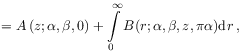
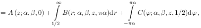
[640.1.4] For ![]() the integral representations read
the integral representations read
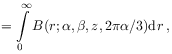 |
(22) | ||||
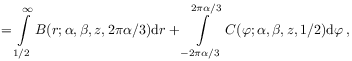 |
(23) |
where the integrands have been defined in eq. (18)–(21) above.
[page 641, §1]
[641.1.1] The integrand ![]() is oscillatory
but bounded over the integration interval.
[641.1.2] Thus the integrals over
is oscillatory
but bounded over the integration interval.
[641.1.2] Thus the integrals over ![]() can be
evaluated numerically using any appropriate quadrature formula.
[641.1.3] We use a robust Gauss-Lobatto quadrature.
can be
evaluated numerically using any appropriate quadrature formula.
[641.1.3] We use a robust Gauss-Lobatto quadrature.
[641.2.1] The integrals over ![]() involve infinite
intervals.
[641.2.2] For given
involve infinite
intervals.
[641.2.2] For given ![]() (resp.
(resp. ![]() ) and accuracy
) and accuracy ![]() we approximate the integrals by truncation.
[641.2.3] The error
we approximate the integrals by truncation.
[641.2.3] The error
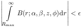 |
(24) |
depends on the truncation point ![]() .
[641.2.4] For
.
[641.2.4] For ![]() we find
we find
![{R_{{\rm max}}}\geq\left\{\begin{array}[]{ll}\max\left\{ 1,\, 2|z|,\,\left(-\ln\frac{\displaystyle\pi\epsilon}{\displaystyle 6}\right)^{\alpha}\right\},&\beta\geq 0\\
\\
\max\left\{(|\beta|+1)^{\alpha},\, 2|z|,\,\left(-2\ln\left(\frac{\displaystyle\pi\epsilon}{\displaystyle 6(|\beta|+2)(2|\beta|)^{{|\beta|}}}\right)\right)^{\alpha}\right\},&\beta<0,\\
\end{array}\right.](mi/mi352.png) |
(25) |
while for ![]() we have
we have
![{R_{{\rm max}}}\geq\left\{\begin{array}[]{ll}\max\left\{ 2^{\alpha},\, 2|z|,\,\left(-2\ln\frac{\displaystyle\pi 2^{\beta}\epsilon}{\displaystyle 12}\right)^{\alpha}\right\},&\beta\geq 0\\
\\
\max\left\{[2(|\beta|+1)]^{\alpha},\, 2|z|,\left[-4\ln\frac{\displaystyle\pi 2^{\beta}\epsilon}{\displaystyle 12\left(|\beta|+2\right)(4|\beta|)^{{|\beta|}}}\right]^{\alpha}\right\},&\beta<0.\end{array}\right.](mi/mi353.png) |
(26) |
2.5 Exponential Asymptotics
[641.3.1] The asymptotic expansions given in eqs. (21) and (22)
on page 210 in Ref. [2] indicate that the
Mittag-Leffler function exhibits a Stokes phenomenon.
[641.3.2] The Stokes lines are the rays ![]() and it was recently shown in [23] that a
Berry-type smoothing applies.
[641.3.3] The exponentially improved asymptotic expansions
will be used here for computing
and it was recently shown in [23] that a
Berry-type smoothing applies.
[641.3.3] The exponentially improved asymptotic expansions
will be used here for computing ![]() for
for ![]() .
[641.3.4] More precisely for
.
[641.3.4] More precisely for ![]() we use the
following exponentially improved
uniform asymptotic expansions [23] :
we use the
following exponentially improved
uniform asymptotic expansions [23] :
| (27) |
for ![]()
| (28) |
for ![]() ,
,
| (29) |
[page 642, §0]
for ![]() with
with ![]() and
and ![]() , and
, and
| (30) |
for ![]() with
with ![]() and
and ![]() .
[642.0.1] Here
.
[642.0.1] Here ![]() is a small number, in practice we use
is a small number, in practice we use
![]() .
[642.0.2] In eqs. (2.5) and (2.5)
.
[642.0.2] In eqs. (2.5) and (2.5)
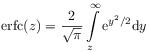 |
(31) |
denotes the complex complementary error function. [642.0.3] Note the difference between eqs. (27)–(2.5) and the expansions in [2, p. 210]. [642.0.4] We take
| (32) |
to truncate the asymptotic series.
[642.0.5] Choosing for ![]() the machine precision we fix the
radius
the machine precision we fix the
radius ![]() in
in ![]() at
at
| (33) |
[642.0.6] The remainder estimates in eqs. (27)–(2.5)
are only valid for a value of ![]() that is chosen in an optimal
sense as in eqs. (32) and (33).
that is chosen in an optimal
sense as in eqs. (32) and (33).
