3 Results
[642.1.1] In this section we present the results of extensive numerical
calculations using an algorithm that is based on the error
estimates developed above.
[642.1.2] Our results give a comprehensive picture of the behaviour
of ![]() in the complex
in the complex ![]() -plane for all values
of the parameters
-plane for all values
of the parameters ![]() ,
, ![]() .
.
3.1 Complex Zeros
[642.2.1] Contrary to the exponential function the Mittag-Leffler functions
exhibit complex zeros denoted as ![]() .
[642.2.2] The complex zeros were studied by Wiman [8] who
found the asymptotic curve along which the zeros
are located for
.
[642.2.2] The complex zeros were studied by Wiman [8] who
found the asymptotic curve along which the zeros
are located for ![]() and showed that
they fall on the negative real axis for all
and showed that
they fall on the negative real axis for all ![]() .
[642.2.3] For real
.
[642.2.3] For real ![]() these zeros come in complex conjugate pairs.
[642.2.4] The pairs are denoted as
these zeros come in complex conjugate pairs.
[642.2.4] The pairs are denoted as ![]() with integers
with integers ![]() where
where ![]() (resp.
(resp. ![]() ) labels zeros in the upper (resp. lower) half plane.
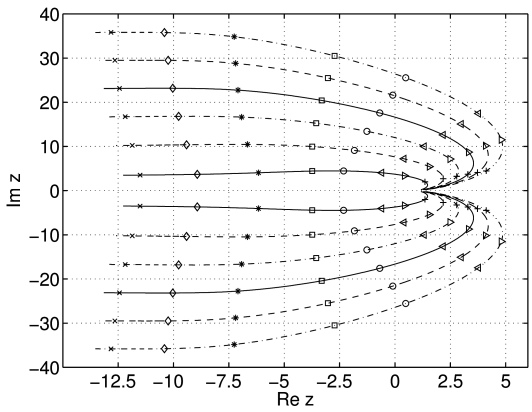
[642.2.5] Figure 1 shows lines that the complex zeros
) labels zeros in the upper (resp. lower) half plane.
[642.2.5] Figure 1 shows lines that the complex zeros
![]() ,
, ![]() of
of ![]() trace out as functions
of
trace out as functions
of ![]() for
for ![]() .
[642.2.6] Figure 1 gives strong
numerical evidence that the distance between
zeros diminishes as
.
[642.2.6] Figure 1 gives strong
numerical evidence that the distance between
zeros diminishes as ![]() .
[642.2.7] Moreover all zeros approach the point
.
[642.2.7] Moreover all zeros approach the point ![]() as
as ![]() .
[642.2.8] This fact seems to have been overlooked until now.
[642.2.9] Of course, for every fixed
.
[642.2.8] This fact seems to have been overlooked until now.
[642.2.9] Of course, for every fixed ![]() the point
the point ![]() is neither
a zero nor an accumulation point of zeros
because the zeros of an entire function must remain isolated.
[642.2.10] The numerical evidence is confirmed analytically.
is neither
a zero nor an accumulation point of zeros
because the zeros of an entire function must remain isolated.
[642.2.10] The numerical evidence is confirmed analytically.
[page 643, §1]
Theorem 3.1.
The zeros ![]() of
of ![]() obey
obey
| (34) |
for all ![]() .
.
[643.0.1] For the proof we note that Wiman showed [8, p. 226]
| (35) |
and further that the number
of zeros with ![]() is given by
is given by
![]() [8, p. 228].
[643.0.2] From this follows that
[8, p. 228].
[643.0.2] From this follows that
| (36) |
for all ![]() .
[643.0.3] Taking the limit
.
[643.0.3] Taking the limit ![]() in (35) and (36)
gives
in (35) and (36)
gives ![]() and
and ![]() for all
for all ![]() .
.
[page 644, §1]
[644.1.1] The theorem states that in the limit ![]() all zeros collapse into a singularity at
all zeros collapse into a singularity at ![]() .
[644.1.2] Next we turn to the limit
.
[644.1.2] Next we turn to the limit ![]() [644.1.3] Of course for
[644.1.3] Of course for ![]() we have
we have ![]() which is free from zeros.
[644.1.4] Figure 1 shows that this is indeed
the case because, as
which is free from zeros.
[644.1.4] Figure 1 shows that this is indeed
the case because, as ![]() , the zeros approach
, the zeros approach ![]() along straight lines parallel to the negative real axis.
[644.1.5] In fact we find
along straight lines parallel to the negative real axis.
[644.1.5] In fact we find
Theorem 3.2.
Let ![]() .
Then the zeros
.
Then the zeros ![]() of
of ![]() obey
obey
| (37) | |||
| (38) |
for all ![]() .
.
[644.1.6] The theorem shows that the phase switches
as ![]() crosses the value
crosses the value ![]() in the sense that minima (valleys)
and maxima (hills) of the Mittag-Leffler
function are exchanged
(see also Figures 7 and
8 below).
in the sense that minima (valleys)
and maxima (hills) of the Mittag-Leffler
function are exchanged
(see also Figures 7 and
8 below).
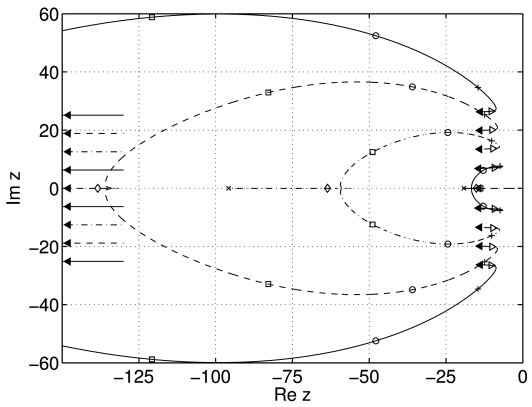
[644.2.1] The location of zeros as function of ![]() for the
case
for the
case ![]() is illustrated in Figure 2.
[644.2.2] Note that with increasing
is illustrated in Figure 2.
[644.2.2] Note that with increasing ![]() more and more pairs of
zeros collapse onto the negative real axis.
[644.2.3] The collapse appears to happen in a continuous manner
(see also Figures 9 and 10
below).
[644.2.4] It is interesting to note that after two conjugate zeros
merge to become a single zero on the negative real axis
this merged zero first moves to the right towards zero and
only afterwards starts to move left towards
more and more pairs of
zeros collapse onto the negative real axis.
[644.2.3] The collapse appears to happen in a continuous manner
(see also Figures 9 and 10
below).
[644.2.4] It is interesting to note that after two conjugate zeros
merge to become a single zero on the negative real axis
this merged zero first moves to the right towards zero and
only afterwards starts to move left towards ![]() .
[644.2.5] This effect can also be seen in Figure 2.
[644.2.6] For
.
[644.2.5] This effect can also be seen in Figure 2.
[644.2.6] For ![]() the zeros
the zeros ![]() all fall
on the negative real axis as can be seen
in Figure 11 below.
[644.2.7] For
all fall
on the negative real axis as can be seen
in Figure 11 below.
[644.2.7] For ![]() all zeros lie on the negative real axis.
all zeros lie on the negative real axis.
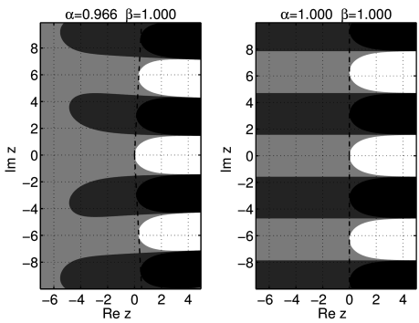
3.2 Contour Lines
[644.3.1] Next we present contour plots for ![]() .
[644.3.2] We use the notation
.
[644.3.2] We use the notation
| (39) | |||
| (40) |
for the contour lines of the real and imaginary part.
[644.3.3] The region ![]() will be coloured white.
[644.3.4] The region
will be coloured white.
[644.3.4] The region ![]() will be coloured black.
[644.3.5] The region
will be coloured black.
[644.3.5] The region ![]() is light gray.
[644.3.6] The region
is light gray.
[644.3.6] The region ![]() is dark gray.
[644.3.7] Thus the contour line
is dark gray.
[644.3.7] Thus the contour line ![]() separates the light gray from dark
gray, the contour
separates the light gray from dark
gray, the contour ![]() separates white from light gray,
and
separates white from light gray,
and ![]() dark gray from black.
[644.3.8] Because
dark gray from black.
[644.3.8] Because ![]() is continuous there exists
in all figures light and dark gray regions between white
and black regions even if the gray regions
cannot be discerned on a figure.
is continuous there exists
in all figures light and dark gray regions between white
and black regions even if the gray regions
cannot be discerned on a figure.

[page 645, §1]
[645.1.1] We begin our discussion with the case ![]() .
Setting
.
Setting ![]() the series (1) defines the function
the series (1) defines the function
| (41) |
for all ![]() .
[645.1.2] This function is not entire, but can be analytically
continued to all of
.
[645.1.2] This function is not entire, but can be analytically
continued to all of ![]() , and
has then a simple pole at
, and
has then a simple pole at ![]() for all
for all ![]() .
[645.1.3] In Figure 3 we show the contour plot
for the case
.
[645.1.3] In Figure 3 we show the contour plot
for the case ![]() ,
, ![]() .
[645.1.4] The contour line
.
[645.1.4] The contour line ![]() is the straight line
is the straight line
![]() separating the left and right half plane.
[645.1.5] The contour line
separating the left and right half plane.
[645.1.5] The contour line ![]() is the boundary circle
of the white disc on the left, while the contour line
is the boundary circle
of the white disc on the left, while the contour line
![]() is the boundary of the black disc on the right.
is the boundary of the black disc on the right.
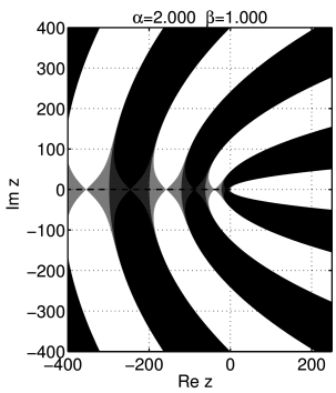
[645.2.1] Having discussed the case ![]() we turn
to the case
we turn
to the case ![]() and note that the limit
and note that the limit
![]() is not continuous.
[645.2.2] For
is not continuous.
[645.2.2] For ![]() the Mittag-Leffler function is an entire function.
[645.2.3] As an example we show the contour plot for
the Mittag-Leffler function is an entire function.
[645.2.3] As an example we show the contour plot for ![]() ,
, ![]() in Figure 4.
[645.2.4] The central white circular lobe extending
[page 646, §0]
to the origin appears to be a remnant of the white disc
in Figure 3.
[646.0.1] They evolve continuously from each other
upon changing
in Figure 4.
[645.2.4] The central white circular lobe extending
[page 646, §0]
to the origin appears to be a remnant of the white disc
in Figure 3.
[646.0.1] They evolve continuously from each other
upon changing ![]() between 0 and 0.2.
[646.0.2] It seems as if the singularity at
between 0 and 0.2.
[646.0.2] It seems as if the singularity at ![]() for
for ![]() had moved along the real axis through the black
circle to
had moved along the real axis through the black
circle to ![]() thereby producing an infinite number of
secondary white and black lobes (or fingers) confined to a
wedge shaped region with opening angle
thereby producing an infinite number of
secondary white and black lobes (or fingers) confined to a
wedge shaped region with opening angle ![]() .
.
[646.1.1] The behaviour of ![]() for
for ![]() is generally
dominated by the wedge
is generally
dominated by the wedge ![]() indicated by dashed lines in Figure 4.
[646.1.2] For
indicated by dashed lines in Figure 4.
[646.1.2] For ![]() the Mittag-Leffler
function grows to infinity as
the Mittag-Leffler
function grows to infinity as ![]() .
[646.1.3] Inside this wedge the function oscillates as a
function of
.
[646.1.3] Inside this wedge the function oscillates as a
function of ![]() .
[646.1.4] For
.
[646.1.4] For ![]() the function decays to zero as
the function decays to zero as
![]() .
[646.1.5] Along the delimiting rays, i.e. for
.
[646.1.5] Along the delimiting rays, i.e. for ![]() ,
the function approaches
,
the function approaches ![]() in an oscillatory fashion.
in an oscillatory fashion.

(The gray level coding is the same as in Figure 3)
[646.2.1] The oscillations inside the wedge are seen as black and
white lobes (or fingers) in Figure 4.
[646.2.2] Each white finger is surrounded by a light gray region.
[646.2.3] Near the tip of the light gray region surrounding a white
finger lie complex zeros of the Mittag-Leffler function.
[646.2.4] The real part ![]() is symmetric with respect to the real axis.
is symmetric with respect to the real axis.
[646.3.1] Contrary to ![]() the contour line
the contour line ![]() consists of infinitely many pieces.
[646.3.2] These pieces will be denoted as
consists of infinitely many pieces.
[646.3.2] These pieces will be denoted as
![]() with
with ![]() located in the
upper (
located in the
upper (![]() ) resp. lower (
) resp. lower (![]() ) half plane.
[646.3.3] The numbering is chosen from left to right, so that
) half plane.
[646.3.3] The numbering is chosen from left to right, so that
![]() separates the light gray region
in the left half plane from the dark gray in the right half plane.
[646.3.4] The line
separates the light gray region
in the left half plane from the dark gray in the right half plane.
[646.3.4] The line ![]() is the boundary of the
light gray region surrounding the first white “finger”
(lobe) in the upper half plane and
is the boundary of the
light gray region surrounding the first white “finger”
(lobe) in the upper half plane and ![]() is its reflection on the real axis.
[646.3.5] Similarly for
is its reflection on the real axis.
[646.3.5] Similarly for ![]() .
[646.3.6] Note that
.
[646.3.6] Note that ![]() seem to encircle the
central white lobe (“bubble”) by going to
seem to encircle the
central white lobe (“bubble”) by going to ![]() parallel to the
imaginary axis.
parallel to the
imaginary axis.
[646.4.1] With increasing ![]() the wedge
the wedge ![]() opens,
the central lobe becomes smaller, the side fingers (or lobes)
grow thicker and begin to extend towards the left half plane.
[646.4.2] At the same time the contour line
opens,
the central lobe becomes smaller, the side fingers (or lobes)
grow thicker and begin to extend towards the left half plane.
[646.4.2] At the same time the contour line ![]() moves
to the left.
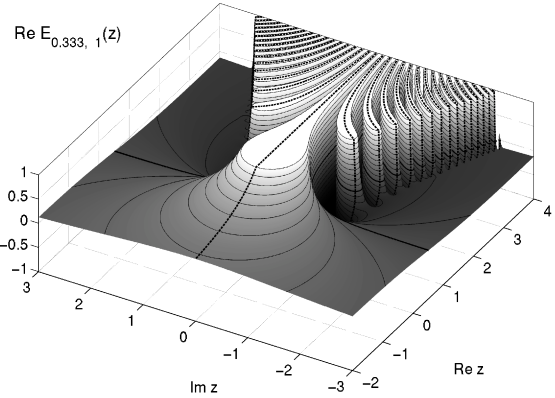
[646.4.3] This is illustrated in a threedimensional plot of
moves
to the left.
[646.4.3] This is illustrated in a threedimensional plot of
![]() in Figure 5.
[646.4.4] In this Figure we have indicated also the complex zeros
as the intersection of
in Figure 5.
[646.4.4] In this Figure we have indicated also the complex zeros
as the intersection of ![]() (shown as thick
solid lines) and
(shown as thick
solid lines) and ![]() (shown as thick
dashed lines).
[646.4.5] At
(shown as thick
dashed lines).
[646.4.5] At ![]() the contours
the contours ![]() cross
the imaginary axis.
cross
the imaginary axis.
[page 647, §1]
[647.1.1] Around ![]() the contours
the contours ![]() osculate the contours
osculate the contours ![]() .
[647.1.2] The osculation eliminates a light gray finger and creates
a dark gray finger.
[647.1.3] In Figure 6
we show the situation before and after the osculation.
[647.1.4] This is the first of an infinity of similar osculations
between
.
[647.1.2] The osculation eliminates a light gray finger and creates
a dark gray finger.
[647.1.3] In Figure 6
we show the situation before and after the osculation.
[647.1.4] This is the first of an infinity of similar osculations
between ![]() and
and ![]() for
for ![]() .
[647.1.5] We estimate the value of
.
[647.1.5] We estimate the value of ![]() for the first
osculation at
for the first
osculation at ![]() .
.
(The gray level coding is the same as in Figure 3)
[647.2.1] For ![]() the dark gray fingers (where
the dark gray fingers (where ![]() )
extend more and more into the left half plane.
[647.2.2] For
)
extend more and more into the left half plane.
[647.2.2] For ![]() the wedge
the wedge ![]() becomes the right half plane
and the lobes or fingers run parallel to the real axis.
[647.2.3] The dark gray fingers, and therefore the oscillations,
now extend to
becomes the right half plane
and the lobes or fingers run parallel to the real axis.
[647.2.3] The dark gray fingers, and therefore the oscillations,
now extend to ![]() .
[647.2.4] The contour lines
.
[647.2.4] The contour lines ![]() degenerate into
degenerate into
| (42) |
i.e. into straight lines parallel to the real axis.
[647.2.5] This case is shown in Figure 7.
[647.2.6] For ![]() with
with ![]() the gray
fingers are again finite.
[647.2.7] This is shown in Figure 8.
the gray
fingers are again finite.
[647.2.7] This is shown in Figure 8.
(The gray level coding is the same as in Figure 3)
(The gray level coding is the same as in Figure 3)
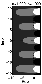
[647.3.1] As ![]() is increased further the fingers grow thicker
and approach each other near the negative real axis.
[647.3.2] For
is increased further the fingers grow thicker
and approach each other near the negative real axis.
[647.3.2] For ![]() the first of an infinite
cascade of osculations appears.
[647.3.3] This is shown in Figure 9.
[647.3.4] The limit
the first of an infinite
cascade of osculations appears.
[647.3.3] This is shown in Figure 9.
[647.3.4] The limit ![]() is illustrated in
Figures 10 and 11.
[647.3.5] Note that the background colour changes from light
gray in Figure 10 to dark gray in
11 in agreement with the discussion
of complex zeros above.
is illustrated in
Figures 10 and 11.
[647.3.5] Note that the background colour changes from light
gray in Figure 10 to dark gray in
11 in agreement with the discussion
of complex zeros above.
(The gray level coding is the same as in Figure 3)
(The gray level coding is the same as in Figure 3)
(The gray level coding is the same as in Figure 3)
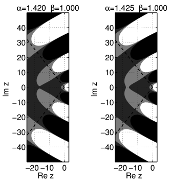
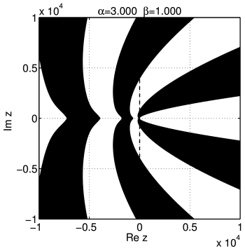
[647.4.1] For ![]() the behaviour changes drastically.
[647.4.2] Figure 12 shows the contour
plot for
the behaviour changes drastically.
[647.4.2] Figure 12 shows the contour
plot for ![]() ,
, ![]() .
[647.4.3] Note the scale of the axes and hence there
are no visible dark or light gray regions.
[647.4.4] The wedge shaped region is absent.
[647.4.5] The rays delimiting the wedge may still be
viewed as if the fingers were following them
in the same way as for
.
[647.4.3] Note the scale of the axes and hence there
are no visible dark or light gray regions.
[647.4.4] The wedge shaped region is absent.
[647.4.5] The rays delimiting the wedge may still be
viewed as if the fingers were following them
in the same way as for ![]() .
[647.4.6] Thus the fingers are more strongly bent
as they approach the negative real axis.
.
[647.4.6] Thus the fingers are more strongly bent
as they approach the negative real axis.
(The gray level coding is the same as in Figure 3)
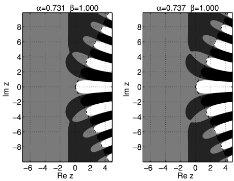
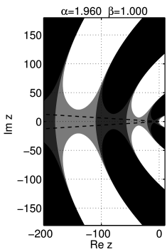
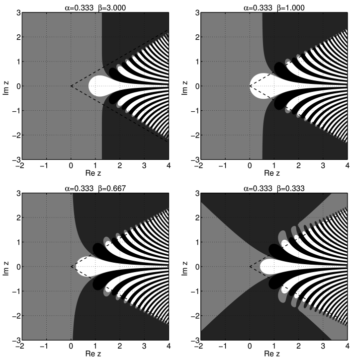
[647.5.1] Now we turn to the cases ![]() choosing
choosing ![]() for illustration.
[647.5.2] For
for illustration.
[647.5.2] For ![]() equation (41) implies that
the central lobe first grows (because
equation (41) implies that
the central lobe first grows (because ![]() diminishes)
and then shrinks as
diminishes)
and then shrinks as ![]() for small values of
for small values of ![]() .
[647.5.3] This is illustrated in the upper left subfigure of
Figure 13.
[647.5.4] For reference the case
.
[647.5.3] This is illustrated in the upper left subfigure of
Figure 13.
[647.5.4] For reference the case ![]() is also shown
in the upper right subfigure of Figure 13.
is also shown
in the upper right subfigure of Figure 13.
(The gray level coding is the same as in Figure 3)
[647.6.1] More interesting behaviour is obtained for ![]() .
[647.6.2] In this case the contours
.
[647.6.2] In this case the contours ![]() stop to run to infinity parallel to the imaginary axis.
[647.6.3] Instead they seem to approach infinity along rays
extending into the negative half axis as illustrated
in the lower left subfigure of Figure 13.
[647.6.4] At the same time a sequence of osculations between
stop to run to infinity parallel to the imaginary axis.
[647.6.3] Instead they seem to approach infinity along rays
extending into the negative half axis as illustrated
in the lower left subfigure of Figure 13.
[647.6.4] At the same time a sequence of osculations between
![]() and
and ![]() begins starting from
begins starting from ![]() .
[647.6.5] One of the last of these osculations can be
seen for
.
[647.6.5] One of the last of these osculations can be
seen for ![]() on the lower right subfigure of
Figure 13.
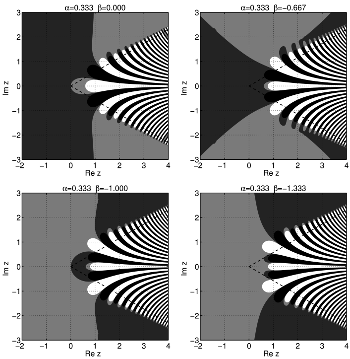
[647.6.6] As
on the lower right subfigure of
Figure 13.
[647.6.6] As ![]() falls below
falls below ![]() the contour
the contour ![]() coalesces with
coalesces with ![]() to form a new large
finite central lobe.
[647.6.7] This new second lobe becomes smaller and retracts towards
the origin for
to form a new large
finite central lobe.
[647.6.7] This new second lobe becomes smaller and retracts towards
the origin for ![]() .
[647.6.8] This can be seen from the upper left subfigure of
Figure 14 where the case
.
[647.6.8] This can be seen from the upper left subfigure of
Figure 14 where the case ![]() is shown.
[647.6.9] As
is shown.
[647.6.9] As ![]() falls below zero the same process of formation
of a new central lobe accompanied by a cascade of
osculations starts again.
[647.6.10] This occurs iteratively whenever
falls below zero the same process of formation
of a new central lobe accompanied by a cascade of
osculations starts again.
[647.6.10] This occurs iteratively whenever ![]() crosses a negative
integer and is a consequence of the poles in
crosses a negative
integer and is a consequence of the poles in ![]() .
.
(The gray level coding is the same as in Figure 3)
