3 Almost invariant states
[631.2.1] Strictly stationary or invariant states [15] are an idealization. [631.2.2] In experiments stationarity is never ideal, but only approximate. [631.2.3] Expectation values are uncertain within the accuracy of the experiment. [631.2.4] Experimental accuracy depends on the response and integration times of the experimental apparatus.
[631.3.1] These experimental restrictions suggest to focus
on a class of states that are stationary
(invariant) only up to a given experimental accuracy ![]() .
[631.3.2] To do so, recall the definition of invariant (stationary) states.
[631.3.3] A state
.
[631.3.2] To do so, recall the definition of invariant (stationary) states.
[631.3.3] A state ![]() is called invariant, if
is called invariant, if
| (15) |
holds for all ![]() and
and ![]() ,
i.e. if the expectation values
,
i.e. if the expectation values ![]() of all observables
of all observables ![]() are constant.
[631.3.4] The set of invariant states
are constant.
[631.3.4] The set of invariant states ![]() over
over ![]() is convex and compact in the weak*-topology [6].
[631.3.5] The same holds for the set of all
states
is convex and compact in the weak*-topology [6].
[631.3.5] The same holds for the set of all
states ![]() .
[631.3.6] Invariant states are fixed points of the adjoint time evolution
.
[631.3.6] Invariant states are fixed points of the adjoint time evolution
![]() as seen from eq. (8).
[631.3.7] Because invariant states are fixed points of
as seen from eq. (8).
[631.3.7] Because invariant states are fixed points of ![]() ,
they are of limited benefit for a proper mathematical formulation
of the problems discussed above.
[631.3.8] Once an orbit in state space reaches an invariant state,
it remains forever in that state and cannot leave it.
,
they are of limited benefit for a proper mathematical formulation
of the problems discussed above.
[631.3.8] Once an orbit in state space reaches an invariant state,
it remains forever in that state and cannot leave it.
[631.4.1] Almost invariant states are based on states
whose expectation values are of
bounded mean oscillation (BMO).
[631.4.2] A state ![]() is called a BMO-state if
all maps
is called a BMO-state if
all maps ![]() have bounded mean oscillation
for all
have bounded mean oscillation
for all ![]() .
[631.4.3] The Banach space
.
[631.4.3] The Banach space ![]() of functions with bounded mean oscillation
on
of functions with bounded mean oscillation
on ![]() is defined as the linear space
is defined as the linear space
| (16) |
where ![]() is the space of locally
integrable functions
is the space of locally
integrable functions ![]() .
[631.4.4] The BMO-norm is defined as
.
[631.4.4] The BMO-norm is defined as
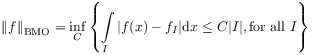 |
(17) |
where ![]() denotes intervals of length
denotes intervals of length ![]() and
and
| (18) |
denotes the average of ![]() over the interval
over the interval ![]() .
[631.4.5] The set of all BMO-states
.
[631.4.5] The set of all BMO-states
| (19) |
is convex by linearity.
[631.4.6] As a subset ![]() of a weak* compact
set it is itself weak* compact.
[631.4.7] Hence a decomposition theory into extremal
BMO-states exists by virtue of the Krein-Milman theorem.
[631.4.8] The set of invariant states is identified through
of a weak* compact
set it is itself weak* compact.
[631.4.7] Hence a decomposition theory into extremal
BMO-states exists by virtue of the Krein-Milman theorem.
[631.4.8] The set of invariant states is identified through
| (20) |
as a subset ![]() .
.
[page 632, §1]
[632.1.1] A BMO-state will be called ![]() -almost invariant
or almost invariant with accuracy
-almost invariant
or almost invariant with accuracy ![]() if the expectation of all observables are
stationary to within experimental accuracy
if the expectation of all observables are
stationary to within experimental accuracy ![]() .
[632.1.2] More precisely, the set
.
[632.1.2] More precisely, the set ![]() of all
of all ![]() -almost
invariant states is defined as
-almost
invariant states is defined as
| (21) |
as a family of subsets of ![]() .
[632.1.3] For small
.
[632.1.3] For small ![]() these states are almost invariant.
[632.1.4] The accuracy
these states are almost invariant.
[632.1.4] The accuracy ![]() measures temporal fluctuations
away from the time average.
measures temporal fluctuations
away from the time average.
[632.2.1] The following inclusions of classes of states used in the following are summarized for orientation and convenience
| (22) |
where ![]() and the set of
KMS-states
and the set of
KMS-states ![]() at inverse temperature
at inverse temperature ![]() are
defined as states
are
defined as states ![]() such that the KMS-condition[16]
such that the KMS-condition[16]
| (23) |
holds for all ![]() and
and ![]() .
[632.2.2] The KMS-states are invariant states for all
.
[632.2.2] The KMS-states are invariant states for all ![]() ,
but KMS-states for different
,
but KMS-states for different ![]() are disjoint [16].
[632.2.3] For
are disjoint [16].
[632.2.3] For ![]() the KMS-states are trace states,
i.e.
the KMS-states are trace states,
i.e. ![]() holds for all
holds for all ![]() .
[632.2.4] Because KMS-states are Gibbs states they are usually
interpreted as equilibrium states with extremal states
corresponding to pure thermodynamic phases [16].
.
[632.2.4] Because KMS-states are Gibbs states they are usually
interpreted as equilibrium states with extremal states
corresponding to pure thermodynamic phases [16].
