2 Problems and Objective
[629.2.1] There are several unsolved problems with the mathematical framework described in the introduction, particularly when the system is infinite. [629.2.2] The following examples of open problems stem from three different areas of theoretical physics.
Open quantum systems: [629.2.3] For open quantum systems with infinite reservoirs
 is the C
 -algebra of bounded operators
on the Hilbert space
-algebra of bounded operators
on the Hilbert space  of the system
  in a suitably chosen GNS-representation.
[629.2.4] The states
in a suitably chosen GNS-representation.
[629.2.4] The states  can be identified with trace class operators on
if
can be identified with trace class operators on
if  denotes the trace operation.
[629.2.5] The unitary time-automorphisms
denotes the trace operation.
[629.2.5] The unitary time-automorphisms
 of are generated by
a Hamiltonian
of are generated by
a Hamiltonian  of
of 
(12) written formally in terms of Hamiltonians
 of
of  ,
,
 of
of  and their interaction
  .
[629.2.6] It is well known[2] that the automorphisms
.
[629.2.6] It is well known[2] that the automorphisms  on
on  do not induce automorphisms on the algebra
  of the open subsystem, because the time evolution will mix
the Hilbert spaces
of the open subsystem, because the time evolution will mix
the Hilbert spaces  and
and  of the system and
the reservoir.
[629.2.7] Even if the initial state is prepared as a product state
of the system and
the reservoir.
[629.2.7] Even if the initial state is prepared as a product state
 the subsystem evolutions defined by
(13a) 
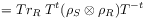
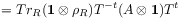
(13b) do not form groups


(14a) 

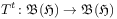
(14b) [page 630, §0] because of memory effects accumulating from the mixing of the system and the reservoir whenever there is nonvanishing interaction [2]. [630.0.1] Here
 denote the density matrices of
the system and the rservoir.
[630.0.2] The trace
denote the density matrices of
the system and the rservoir.
[630.0.2] The trace  integrates out
the reservoir degrees of freedom.
integrates out
the reservoir degrees of freedom.Classical dynamical systems: [630.0.3] In classical systems it is well known [14] that the orbits in the abelian algebra
 of functions on phase space
cannot always be defined for all
of functions on phase space
cannot always be defined for all  and for all initial
conditions
and for all initial
conditions  in the thermodynamics limit.
[630.0.4] The integration of eq. (1) does not generally give
a dynamical flow of time for all initial conditions and
the problem is to find sufficiently large subsets of
such that catastrophic behavior is absent and a unique
orbit exists for all .
in the thermodynamics limit.
[630.0.4] The integration of eq. (1) does not generally give
a dynamical flow of time for all initial conditions and
the problem is to find sufficiently large subsets of
such that catastrophic behavior is absent and a unique
orbit exists for all .Quantum field theory: [630.0.5] For quantum field theories or infinite systems the Stone-von Neumann uniqueness breaks down. [630.0.6] Haags theorem shows that the determination of a suitable representation of the canonical commutation relations becomes a dynamical problem, if the vacuum states for different couplings are different. [630.0.7] Non-normal states arise that yield representations assigning different values to global observables like densities. [630.0.8] Due to the problem of inequivalent representations it is not possible to represent the time evolution as a group of unitary transformation within a single representation, because the representation algebra may change into an inequivalent representation as time evolves.
[630.0.9] One objective of this paper is to suggest that these three open problems are, in fact, related to each other, even though they seem to be unrelated at first sight.
[630.1.1] The present article suggests that the common denominator of problems 2-2 associated with the mathematical framework described in the introduction is the concept of time flow as a translation, implicitly assumed on the left hand side of Equation (1). [630.1.2] The common origin of problems 2-2 emerges from studying the following two general questions associated with Equation (1).
Problem 1.
[630.1.3] Are there global solutions of equation (1),
i.e. solutions for all ![]() ?
?
[630.1.4] If global solutions and hence a group of *-automorphisms on
![]() exist, then
this implies a continuous time evolution for all states
exist, then
this implies a continuous time evolution for all states
![]() .
[630.1.5] This means a time evolution independent of the state,
which is not to be expected for general infinite
systems without rescaling time.
[630.1.6] Rescaling of time is also expected to be necessary
for establishing hydrodynamic limits governing invariant
states.
.
[630.1.5] This means a time evolution independent of the state,
which is not to be expected for general infinite
systems without rescaling time.
[630.1.6] Rescaling of time is also expected to be necessary
for establishing hydrodynamic limits governing invariant
states.
Problem 2.
[630.1.7] If global solutions of equation (1) exist, how can invariant solutions still change with time?
[630.1.8] Local stationarity (invariance) in time arises from the underlying dynamics. [630.1.9] Local stationarity in time is necessary, if thermodynamic observables such as temperature, pressure or densities are to provide an approximate representation of the physical system that changes slowly on long time scales. [630.1.10] Hence one has to study the set of stationary states that are invariant under the time evolution. [630.1.11] If the thermodynamic observables change then there must exist many invariant states and many possible time averages, i.e. the time averages are not unique.
[page 631, §1] [631.1.1] The objective of this paper is to introduce a framework in which questions concerning the abundance of time-invariant states and their embedding in the set of all states can be posed mathematically in a proper way.
