7 Results
[635.1.1] The time evolution of almost invariant states can
be defined by the addition of random recurrence times.
[635.1.2] Let ![]() be the probability density of the sum
be the probability density of the sum
| (40) |
of ![]() independent
and identically-distributed random
recurrence times
independent
and identically-distributed random
recurrence times ![]() .
[635.1.3] Let
.
[635.1.3] Let ![]() from Equation (39)
be the common probability density of all
from Equation (39)
be the common probability density of all ![]() .
[635.1.4] Then, with
.
[635.1.4] Then, with ![]() and
and ![]() ,
,
| (41) |
is an ![]() -fold convolution of the discrete
recurrence time density in Equation (39).
[635.1.5] The family of distributions
-fold convolution of the discrete
recurrence time density in Equation (39).
[635.1.5] The family of distributions ![]() obeys
obeys
| (42) |
for all ![]() , and the discrete analogue of
Equation (5)
, and the discrete analogue of
Equation (5)
| (43) |
holds for all ![]() .
[635.1.6] Because the individual states in
.
[635.1.6] Because the individual states in ![]() are indistinguishable
within the given accuracy
are indistinguishable
within the given accuracy ![]() , but may evolve very
differently in time, it is natural to define the duration
of time needed for the first recurrence (a single time step) as an average
, but may evolve very
differently in time, it is natural to define the duration
of time needed for the first recurrence (a single time step) as an average
| (44) |
over recurrence times.
[635.1.7] If a macroscopic time evolution with a rescaled
time exists, then one has to rescale the sums
![]() and the iterations
and the iterations
| (45) |
in the limit ![]() with suitable norming constants
with suitable norming constants ![]() .
.
Theorem 3.
[635.1.8] Let ![]() be the probability density of
be the probability density of ![]() specified above in (41).
[635.1.9] If the distributions of
specified above in (41).
[635.1.9] If the distributions of ![]() converge
to a limit as
converge
to a limit as ![]() for suitable norming constants
for suitable norming constants ![]() ,
then there exist constants
,
then there exist constants ![]() and
and ![]() ,
such that
,
such that
| (46) |
[page 636, §0] where:
| (47) |
if ![]() diverges, while
diverges, while
| (48) |
if ![]() converges.
[636.0.1] For
converges.
[636.0.1] For ![]() , the function
, the function ![]() is
is ![]() .
[636.0.2] For
.
[636.0.2] For ![]() , the function
, the function ![]() for
for ![]() and
and
| (49) |
for ![]() .
.
Proof.
[636.1.1] The existence of a limiting distribution for ![]() is known to be equivalent to the stability of the limit [18].
[636.1.2] If the limit distribution is nondegenerate,
this implies that
the rescaling constants
is known to be equivalent to the stability of the limit [18].
[636.1.2] If the limit distribution is nondegenerate,
this implies that
the rescaling constants ![]() have the form
have the form
| (50) |
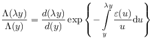
where ![]() is a slowly varying function [19],
defined by the requirement that
is a slowly varying function [19],
defined by the requirement that
| (51) |
holds for all ![]() .
[636.1.3] That the number
.
[636.1.3] That the number ![]() obeys Equation (47)
is proven in [18] (p. 179).
[636.1.4] It is bounded
as
obeys Equation (47)
is proven in [18] (p. 179).
[636.1.4] It is bounded
as ![]() , because the rescaled random
variables
, because the rescaled random
variables ![]() are positive.
are positive.
[636.2.1] To prove Equation (46), note that
the characteristic function of ![]() is
the
is
the ![]() -th power
-th power
| (52) |
because the characteristic functions
![]() of
of ![]() are identical for all
are identical for all ![]() .
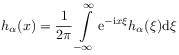
[636.2.2] Inverse Fourier transformation gives:
.
[636.2.2] Inverse Fourier transformation gives:
![\displaystyle p_{N}(k)=\frac{1}{2\pi}\int\limits _{{-\pi}}^{{\pi}}\mathrm{e}^{{-\mathrm{i}\xi k}}\left[p(\xi)\right]^{N}\mathrm{d}\xi=\frac{\tau}{2\pi D_{N}D^{{1/\alpha}}}\int\limits _{{-\pi D_{N}D^{{1/\alpha}}}}^{{\pi D_{N}D^{{1/\alpha}}}}\mathrm{e}^{{-\mathrm{i}\xi x}}\left[p\left(\frac{\xi\tau}{D_{N}D^{{1/\alpha}}}\right)\right]^{N}\mathrm{d}\xi](mi/mi269.png) |
(53) |
where:
| (54) |
and ![]() was substituted with
was substituted with ![]() .
[636.2.3] Let
.
[636.2.3] Let ![]() denote the characteristic function of
denote the characteristic function of
![]() , so that
, so that
 |
(55) |
holds.
[page 637, §1]
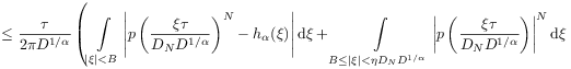
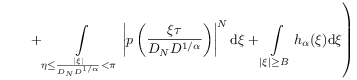
[637.1.1] Following [20],
the difference ![]() in (46) can be
decomposed and bounded from above as
in (46) can be
decomposed and bounded from above as
![\displaystyle=\frac{\tau}{2\pi D^{{1/\alpha}}}\left|\int\limits _{{-\pi D_{N}D^{{1/\alpha}}}}^{{\pi D_{N}D^{{1/\alpha}}}}\mathrm{e}^{{-\mathrm{i}\xi x}}\left[p\left(\frac{\xi\tau}{D_{N}D^{{1/\alpha}}}\right)\right]^{N}\mathrm{d}\xi-\int\limits _{{-\infty}}^{{\infty}}\mathrm{e}^{{-\mathrm{i}\xi x}}\ h_{\alpha}(\xi)\mathrm{d}\xi\right|](mi/mi239.png) |
|||
![\displaystyle=\frac{\tau}{2\pi D^{{1/\alpha}}}\left|\;\int\limits _{{|\xi|<B}}\mathrm{e}^{{-\mathrm{i}\xi x}}\left[p\left(\frac{\xi\tau}{D_{N}D^{{1/\alpha}}}\right)^{N}-h_{\alpha}(\xi)\right]\mathrm{d}\xi+\int\limits _{{B\leq|\xi|<\eta D_{N}D^{{1/\alpha}}}}\mathrm{e}^{{-\mathrm{i}\xi x}}\left[p\left(\frac{\xi\tau}{D_{N}D^{{1/\alpha}}}\right)^{N}-h_{\alpha}(\xi)\right]\mathrm{d}\xi\right.](mi/mi346.png) |
|||
![\displaystyle\qquad\left.+\int\limits _{{\eta\leq\frac{|\xi|}{D_{N}D^{{1/\alpha}}}<\pi}}\mathrm{e}^{{-\mathrm{i}\xi x}}\left[p\left(\frac{\xi\tau}{D_{N}D^{{1/\alpha}}}\right)^{N}-h_{\alpha}(\xi)\right]\mathrm{d}\xi-\int\limits _{{|\xi|\geq\pi D_{N}D^{{1/\alpha}}}}\mathrm{e}^{{-\mathrm{i}\xi x}}\ h_{\alpha}(\xi)\mathrm{d}\xi\right|](mi/mi265.png) |
|||
 |
|||
 |
(56) |
with constants ![]() to be specified below.
[637.1.2] The terms involving
to be specified below.
[637.1.2] The terms involving ![]() from the second and third
integral have been absorbed in the fourth integral.
[637.1.3] The four integrals are now discussed further individually.
from the second and third
integral have been absorbed in the fourth integral.
[637.1.3] The four integrals are now discussed further individually.
[637.2.1] The first integral converges uniformly to zero for
![]() , because
, because
![]() belongs to the domain of attraction
of a stable law with index
belongs to the domain of attraction
of a stable law with index ![]() , as already noted above.
, as already noted above.
[637.3.1] To estimate the second integral, note that the characteristic
function ![]() belongs to the domain of attraction
for index
belongs to the domain of attraction
for index ![]() if and only if it behaves for
if and only if it behaves for ![]() as [20]
as [20]
| (57) |
where ![]() and
and ![]() is a slowly varying function at infinity obeying
is a slowly varying function at infinity obeying
| (58) |
[637.3.2] By the representation
theorem for slowly varying functions ([21] p. 12),
there exist functions ![]() and
and ![]() ,
such that the function
,
such that the function ![]() can be represented as
can be represented as
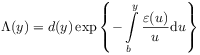 |
(59) |
[page 638, §0]
for some ![]() where
where ![]() is measurable and
is measurable and
![]() , as well as
, as well as ![]() hold for
hold for ![]() .
[638.0.1] As a consequence
.
[638.0.1] As a consequence
 |
(60) |
so that with ![]() and
and ![]()
| (61) |
is obtained for ![]() .
[638.0.2] Therefore, there exists for any
.
[638.0.2] Therefore, there exists for any ![]() a positive number
a positive number
![]() independent of
independent of ![]() , such that
, such that
| (62) |
for sufficiently large ![]() .
[638.0.3] If
.
[638.0.3] If ![]() is sufficiently large,
it is then possible to choose an
is sufficiently large,
it is then possible to choose an ![]() (and find
(and find ![]() ), such that
), such that
 |
(63) |
and this converges to zero for ![]() .
.
[638.1.1] The third integral is estimated by noting that
![]() for
for ![]() .
[638.1.2] Hence, there is a positive constant
.
[638.1.2] Hence, there is a positive constant ![]() , such that
, such that
| (64) |
for ![]() .
[638.1.3] Consequently, with Equation (50),
.
[638.1.3] Consequently, with Equation (50),
![\displaystyle\int\limits _{{\eta\leq\frac{|\xi|}{D_{N}D^{{1/\alpha}}}<\pi}}\left|p\left(\frac{\xi\tau}{D_{N}D^{{1/\alpha}}}\right)\right|^{N}\mathrm{d}\xi\leq 2\pi\mathrm{e}^{{-cN}}\left[N\Lambda(N)D\right]^{{1/\alpha}}](mi/mi250.png) |
(65) |
converges to zero as ![]() .
.
[638.3.1] Equation (46) implies
| (66) |
for sufficiently large ![]() and all
and all ![]() .
[638.3.2] Inserting this into Equation (45) gives
.
[638.3.2] Inserting this into Equation (45) gives
| (67) |
[page 639, §0]
[639.0.1] For ![]() , the average return time
, the average return time
![]() is proportional to the discretization
is proportional to the discretization ![]() .
[639.0.2] In the case
.
[639.0.2] In the case ![]() , the average
time
, the average
time ![]() for return into
the set
for return into
the set ![]() in a single step diverges.
[639.0.3] This suggests an infinite rescaling of time as
in a single step diverges.
[639.0.3] This suggests an infinite rescaling of time as ![]() for
for ![]() .
[639.0.4] This rescaling of time combined with
.
[639.0.4] This rescaling of time combined with
![]() was called the ultra-long-time limit in [22].
[639.0.5] In the ultra-long-time limit
was called the ultra-long-time limit in [22].
[639.0.5] In the ultra-long-time limit ![]() with:
with:
| (68) |
one finds from Equation (67) the result
![\displaystyle\lim _{{{\tau\to\infty,N\to\infty}\atop{[N\Lambda(N)D]^{{1/\alpha}}/\tau=a}}}\mathscr{S}^{{-N}}\approx\sum _{{k=1}}^{\infty}h_{\alpha}\left(\frac{k}{a}\right)\;\mathscr{T}^{{-ka}}\;\frac{[k-(k-1)]}{a}\approx\int\limits _{0}^{\infty}h_{\alpha}\left(x\right)\;\mathscr{T}^{{-xa}}\;\mathrm{d}x](mi/mi257.png) |
(69) |
for sufficiently large ![]() and
and ![]() .
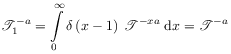
[639.0.6] The limit gives rise to
a family of one-parameter semigroups
.
[639.0.6] The limit gives rise to
a family of one-parameter semigroups ![]() (with family index
(with family index ![]() and parameter
and parameter ![]() )
of ultra-long-time evolution operators
)
of ultra-long-time evolution operators
![\displaystyle\lim _{{{\tau\to\infty,N\to\infty}\atop{[N\Lambda(N)D]^{{1/\alpha}}/\tau=a}}}\mathscr{S}^{{-N}}=\mathscr{T}^{{-a}}_{{\alpha}}=\int\limits _{0}^{\infty}h_{\alpha}\left(x\right)\;\mathscr{T}^{{-xa}}\;\mathrm{d}x](mi/mi256.png) |
(70) |
which are convolutions instead of translations.
[639.0.7] Note that
![]() because
because
![]() and
and ![]() .
[639.0.8] The rescaled age evolutions
.
[639.0.8] The rescaled age evolutions ![]() are called fractional time evolutions, because
their infinitesimal generators are
fractional time derivatives [22, 23].
are called fractional time evolutions, because
their infinitesimal generators are
fractional time derivatives [22, 23].
[639.1.1] The result shows that a proper mathematical
formulation of local stationarity requires a generalization of the
left-hand side in Equation (1), because
Equation (1) assumes implicitly a translation along the orbit.
[639.1.2] In general, the integration of infinitesimal
system changes leads to convolutions instead
of just translations along the orbit [22, 23].
[639.1.3] Of course, translations are a special case of
convolutions, to which they reduce in the
case when the parameter ![]() approaches unity.
[639.1.4] For
approaches unity.
[639.1.4] For ![]() , one finds
, one finds
| (71) |
and therefore
 |
(72) |
is a right translation.
[639.1.5] Here, ![]() is an age or duration.
[639.1.6] This shows that also the special case of
induced right translations does not give
a group, but only a semigroup.
is an age or duration.
[639.1.6] This shows that also the special case of
induced right translations does not give
a group, but only a semigroup.
