2.3 Physical Introduction to Fractional Derivatives

[page 46, §1]

2.3.1 Basic Questions

[46.1.1] An introduction to fractional derivatives would be incomplete without an introduction to applications. [46.1.2] In the past fractional calculus has been used predominantly as a convenient calculational tool [76, 89, 26]. [46.1.3] A well known example is Riesz’ interpolation method for solving the wave equation [20]. [46.1.4] In recent times, however, fractional differential equations appear as ‘‘generalizations’’ of more or less fundamental equations of physics [18, 3, 90, 12, 104, 43, 60, 46, 54, 52, 56, 55, 58, 23, 91, 102, 129, 119]. [46.1.5] The idea is that physical phenomena can be described by fractional differential equations. [46.1.6] This practice raises at least two fundamental questions:

[46.1.7] Are mathematical models with fractional derivatives consistent with the fundamental laws and fundamental symmetries of nature ?
[46.1.8] How can the fractional order $\alpha$ of differentiation be observed or how does a fractional derivative emerge from concrete models ?

[46.1.9] Both questions will be addressed here. [46.1.10] The answer to the first question is provided by the theory of fractional time evolutions [43, 47], the answer to the second question by anomalous subdiffusion [60, 46].

2.3.2 Fractional Space

[46.2.1] Fractional derivatives are nonlocal operators. [46.2.2] Nevertheless, numerous authors have proposed fractional differential equations involving fractional spatial derivatives. [46.2.3] Particularly popular are fractional powers of the Laplace operator due to the well known work of Riesz, Feller and Bochner [97, 13, 27]. The nonlocality of fractional spatial derivatives raises serious (largely) unresolved physical problems.

[46.3.1] As an illustration of the problem with spatial fractional derivatives consider the one dimensional potential equation for functions $f\in C^{{2}}(\mathbb{R})$

$\frac{\mathrm{d}^{2}}{\mathrm{d}x^{2}}f(x)=0,\quad x\in\mathbb{G}$

(2.136)

on the open interval $\mathbb{G}=]a,b[$ with boundary conditions $f(a)=0,f(b)=0$ with $a<b$ . A solution of this boundary value problem is $f(x)=0$ with $x\in\mathbb{G}$ . [46.3.2] This trivial solution remains unchanged as long as the boundary values $f(a)=f(b)=0$ remain unperturbed. [46.3.3] All functions $f\in C^{{2}}(\mathbb{R})$ that vanish on $[a,b]$ are solutions of the boundary value problem. [46.3.4] In particular, the boundary

[page 47, §0] specification

$\displaystyle f(x)=0,\quad\text{for~}x\in\mathbb{R}\setminus\mathbb{G}$

(2.137)

and the perturbed boundary specification

$f(x)=g(x),\quad\text{for~}x\in\mathbb{R}\setminus\mathbb{G}$

(2.138)

with $g\geq 0$ and $\mathrm{supp}\, g\cap[a,b]=\emptyset$ have the same trivial solution $f=0$ in $\mathbb{G}$ . [47.0.1] The reason is that $\mathrm{d}^{2}/\mathrm{d}x^{2}$ is a local operator.

[47.1.1] Consider now a fractional generalization of (2.136) that arises for example as the stationary limit of (Bochner-Levy) fractional diffusion equations with a fractional Laplace operator [13]. [47.1.2] Such a onedimensional fractional Laplace equation reads

$\mathrm{R}^{{\alpha}}f(x)=0,$

(2.139)

where $\mathrm{R}^{{\alpha}}$ is a Riesz fractional derivative of order $0<\alpha<1$ . [47.1.3] For the boundary specification (2.137) it has the same trivial solution $f(x)=0$ for all $x\in\mathbb{G}$ . [47.1.4] But this solution no longer applies for the perturbed boundary specification (2.138). [47.1.5] In fact, assuming (2.138) for $x\in\mathbb{R}\setminus\mathbb{G}$ and $f(x)=0$ for $x\in\mathbb{G}$ now yields $(\mathrm{R}^{{\alpha}}f)(x)\neq 0$ for all $x\in\mathbb{G}$ . [47.1.6] The exterior $\mathbb{R}\setminus\mathbb{G}$ of the domain $\mathbb{G}$ cannot be isolated from the interior of $\mathbb{G}$ using classical boundary conditions. [47.1.7] The reason is that $\mathrm{R}^{{\alpha}}$ is a nonlocal operator.

[47.2.1] Locality in space is a basic and firmly established principle of physics (see e.g. [115, 35]). [47.2.2] Of course, one could argue that relativistic effects are negligible, and that fractional spatial derivatives might arise as an approximate phenomenological model describing an underlying physical reality that obeys spatial locality. [47.2.3] However, spatial fractional derivatives imply not only action at a distance. [47.2.4] As seen above, they imply also that the exterior domain cannot be decoupled from the interior by conventional walls or boundary conditions. [47.2.5] This has far reaching consequences for theory and experiment. [47.2.6] In theory it invalidates all arguments based on surface to volume ratios becoming negligible in the large volume limit. [47.2.7] This includes many concepts and results in thermodynamics and statistical physics that depend on the lower dimensionality of the boundary. [47.2.8] Experimentally it becomes difficult to isolate a system from its environment. [47.2.9] Fractional diffusion would never come to rest inside a vessel with thin rigid walls unless the equilibrium concentration prevails also outside the vessel. [47.2.10] A fractionally viscous fluid at rest inside a container with thin rigid walls would have to start to move when the same fluid starts flowing outside the vessel. [47.2.11] It seems therefore difficult to reconcile nonlocality in space with theory and experiment.

[page 48, §1]

2.3.3 Fractional Time

2.3.3.1 Basic Questions

[48.1.1] Nonlocality in time, unlike space, does not violate basic principles of physics, as long as it respects causality [49, 48, 43, 47, 54]. [48.1.2] In fact, causal nonlocality in time is a common nonequilibrium phenomenon known as history dependence, hysteresis and memory. [48.2.1] Theoretical physics postulates time translation invariance as a fundamental symmetry of nature. [48.2.2] As a consequence energy conservation is fundamental, and the infinitesimal generator of time translations is a first order time derivative. [48.2.3] Replacing integer order time derivatives with fractional time derivatives raises at least three basic questions:

[48.2.4] What replaces time translations as the physical time evolution ?
[48.2.5] Is the nonlocality of fractional time derivatives consistent with the laws of nature ?
[48.2.6] Is the asymmetry of fractional time derivatives consistent with the laws of nature ?

[48.2.7] These questions as well as ergodicity breaking, stationarity, long time limits and temporal coarse grainig were discussed first within ergodic theory [49, 48, 47] and later from a general perspective in [54].

[48.3.1] The third question requires special remarks because irreversibility is a longstanding and controversial subject [71]. [48.3.2] The problem of irreversibility may be formulated briefly in two ways.

Definition 2.20 (The normal irreversibility problem)

[48.4.1] Assume that time is reversible. Explain how and why time irreversible equations arise in physics.

Definition 2.21 (The reversed irreversibility problem)

[48.5.1] Assume that time is irreversible. Explain how and why time reversible equations arise in physics.

[48.6.1] While the normal problem has occupied physicists and mathematicians for more than a century, the reversed problem was apparently first formulated in [59]. [48.6.2] Surprisingly, the reversed irreversibility problem has a clear and quantitiative solution within the theory of fractional time. [48.6.3] The solution is based on the simple postulate that every time evolution of a physical system is irreversible. [48.6.4] It is not possible to repeat an experiment in the past [59]. [48.6.5] This empiricial fact seems to reflect a fundamental law of nature that rivals the law of energy conservation.

[48.7.1] The mathematical concepts corresponding to irreversible time evolutions are operator semigroups and abstract Cauchy problems [15, 93]. [48.7.2] The following brief introduction to fractional time evolutions (sections 2.3.3.2–2.3.3.8) is in large parts identical to the brief exposition in [59]. [48.7.3] For more details see [54].

[page 49, §1]

2.3.3.2 Time Evolution

[49.1.1] A physical time evolution $\{ T({\Delta t}):0\leq{\Delta t}<\infty\}$ is defined as a one-parameter family (with time parameter ${\Delta t}$ ) of bounded linear time evolution operators $T({\Delta t})$ on a Banach space $B$ . [49.1.2] The parameter ${\Delta t}$ represents time durations. The one-parameter family fulfills the conditions

$\displaystyle[T({\Delta t}_{1})T({\Delta t}_{2})f](t_{0})$	$\displaystyle=[T({\Delta t}_{1}+{\Delta t}_{2})f](t_{0})$		(2.140)
$\displaystyle(t_{0})$	$\displaystyle=f(t_{0})$		(2.141)

for all ${\Delta t}_{1},{\Delta t}_{2}\geq 0$ , $t_{0}\in\mathbb{R}$ and $f\in B$ . [49.1.3] The elements $f\in B$ represent time dependent physical observables, i.e. functions on the time axis $\mathbb{R}$ . [49.1.4] Note that the argument ${\Delta t}\geq 0$ of $T({\Delta t})$ has the meaning of a time duration, while $t\in\mathbb{R}$ in $f(t)$ means a time instant. [49.1.5] Equations (2.140) and (2.141) define a semigroup. [49.1.6] The inverse elements $T(-{\Delta t})$ are absent. [49.1.7] This reflects the fundamental difference between past and future.

[49.2.1] The linear operator $\mathrm{A}$ defined as

$\mathrm{A}f=\underset{{\Delta t}\to 0+}{\text{s-lim}}\,\frac{T({\Delta t})f-f}{{\Delta t}}$

(2.142)

with domain

$D(\mathrm{A})=\left\{ f\in B:\underset{{\Delta t}\to 0+}{\text{s-lim}}\,\frac{T({\Delta t})f-f}{{\Delta t}}\;{\rm exists}\right\}$

(2.143)

is called the infinitesimal generator of the semigroup. [49.2.2] Here $\underset{}{\text{s-lim}}\, f=g$ is the strong limit and means $\lim\| f-g\|=0$ in the norm of $B$ as usual.

2.3.3.3 Continuity

[49.3.1] Physical time evolution is continuous. [49.3.2] This requirement is represented mathematically by the assumption that

$\underset{{\Delta t}\to 0}{\text{s-lim}}\, T({\Delta t})f=f$

(2.144)

holds for all $f\in B$ , where $\underset{}{\text{s-lim}}\,$ is again the strong limit. [49.3.3] Semigroups of operators satisfying this condition are called strongly continuous or $C^{0}$ -semigroups [15, 93]. [49.3.4] Strong continuity is weaker than uniform continuity and has become recognized as an important continuity concept that covers most applications [2].

2.3.3.4 Homogeneity

[49.4.1] Homogeneity of time means two different requirements: [49.4.2] Firstly, it requires that observations are independent of a particular instant or position in

[page 50, §0] time. [50.0.1] Secondly, it requires arbitrary divisibility of time durations and self-consistency for the transition between time scales.

[50.1.1] Independence of physical processes from their position on the time axis requires that physical experiments are reproducible if they are ceteris paribus shifted in time. [50.1.2] The first requirement, that the start of an experiment can be shifted, is expressed mathematically as the requirement of invariance under time translations. [50.1.3] As a consequence one demands commutativity of the time evolution with time translations in the form

$[\mathsf{T}({\tau})T({\Delta t})f](t_{0})=[T({\Delta t})\mathsf{T}({\tau})f](t_{0})=[T({\Delta t})f](t_{0}-\tau)$

(2.145)

for all ${\Delta t}\geq 0$ und $t_{0},\tau\in\mathbb{R}$ . [50.1.4] Here the translation operator $\mathsf{T}(t)$ is defined by

$\mathsf{T}({\tau})f(t_{0})=f(t_{0}-\tau).$

(2.146)

[50.1.5] Note that $\tau\in\mathbb{R}$ is a time shift, not a duration. [50.1.6] It can also be negative. Physical experiments in the past have the same outcome as in the present or in the future. [50.1.7] Outcomes of past experiments can be studied in the present with the help of documents (e.g. a video recording), irrespective of the fact that the experiment cannot be repeated in the past.

[50.2.1] The second requirement of homogeneity is homogeneous divisibility. [50.2.2] The semigroup property (2.140) implies that for ${\Delta t}>0$

$T({\Delta t})...T({\Delta t})=\left[T({\Delta t})\right]^{n}=T(n{\Delta t})$

(2.147)

holds. [50.2.3] Homogeneous divisibility of a physical time evolution requires that there exist rescaling factors $D_{n}$ for ${\Delta t}$ such that with ${\Delta t}=\overline{{\Delta t}}/D_{n}$ the limit

$\lim _{{n\to\infty}}T(n\overline{{\Delta t}}/D_{n})={\overline{T}}(\overline{{\Delta t}})$

(2.148)

exists und defines a time evolution ${\overline{T}}(\overline{{\Delta t}})$ . [50.2.4] The limit $n\to\infty$ corresponds to two simultaneous limits $n\to\infty,{\Delta t}\to 0$ , and it corresponds to the passage from a microscopic time scale ${\Delta t}$ to a macroscopic time scale $\overline{{\Delta t}}$ .

2.3.3.5 Causality

[50.3.1] Causality of the physical time evolution requires that the values of the image function $g(t)=(T({\Delta t})f)(t)$ depend only upon values $f(s)$ of the original function with time instants $s<t$ .

2.3.3.6 Fractional Time Evolution

[50.4.1] The requirement (2.145) of homogeneity implies that the operators $T({\Delta t})$ are convolution operators [128, 114]. Let $T$ be a bounded linear operator on $L^{1}(\mathbb{R})$ that commutes with time translations, i.e. that fulfills eq. (2.145). [50.4.2] Then there

[page 51, §0] exists a finite Borel measure $\mu$ such that

$(Tf)(s)=(\mu*f)(s)=\int f(s-x)\mu(\mathrm{d}x)$

(2.149)

holds [128],[114, p.26]. [51.0.1] Applying this theorem to physical time evolution operators $T({\Delta t})$ yields a convolution semigroup $\mu _{{\Delta t}}$ of measures $T({\Delta t})f(t)=(\mu _{{\Delta t}}*f)(t)$

$\mu _{{{\Delta t}_{1}}}*\mu _{{{\Delta t}_{2}}}=\mu _{{{\Delta t}_{1}+{\Delta t}_{2}}}$

(2.150)

with ${\Delta t}_{1},{\Delta t}_{2}\geq 0$ . [51.0.2] For ${\Delta t}=0$ the measure $\mu _{0}$ is the Dirac-measure concentrated at $0$ .

[51.1.1] The requirement of causality implies that the support $\mathrm{supp}\,\mu _{{\Delta t}}\subset\mathbb{R}_{+}=[0,\infty)$ of the semigroup is contained in the positive half axis.

[51.2.1] The convolution semigroups with support in the positive half axis $[0,\infty)$ can be characterized completely by Bernstein functions [10]. [51.2.2] An arbitrarily often differentiable function $b:(0,\infty)\to\mathbb{R}$ with continuous extension to $[0,\infty)$ is called Bernstein function if for all $x\in(0,\infty)$

$\displaystyle b(x)$	$\displaystyle\geq 0$		(2.151)
$\displaystyle(-1)^{n}\frac{\mathrm{d}^{n}b(x)}{\mathrm{d}x^{n}}$	$\displaystyle\leq 0$		(2.152)

holds for all $n\in\mathbb{N}$ . [51.2.3] Bernstein functions are positive, monotonously increasing and concave.

[51.3.1] The characterization is given by the following theorem [10, p.68]. [51.3.2] There exists a one-to-one mapping between the convolution semigroups $\{\mu _{t}:t\geq 0\}$ with support on $[0,\infty)$ and the set of Bernstein functions $b:(0,\infty)\to\mathbb{R}$ [10]. [51.3.3] This mapping is given by

$\int _{0}^{\infty}e^{{-ux}}\mu _{{\Delta t}}(\mathrm{d}x)=e^{{-{\Delta t}b(u)}}$

(2.153)

with ${\Delta t}>0$ and $u>0$ .

[51.4.1] The requirement of homogeneous divisibility further restricts the set of admissible Bernstein functions. [51.4.2] It leaves only those measures $\mu$ that can appear as limits

$\lim _{{n\to\infty,{\Delta t}\to 0}}\underbrace{\mu _{{\Delta t}}*...*\mu _{{\Delta t}}}_{{n\;\;{\rm factors}}}=\lim _{{n\to\infty}}\mu _{{n\overline{{\Delta t}}/D_{n}}}={\overline{\mu}}_{{\overline{{\Delta t}}}}.$

(2.154)

[51.4.3] Such limit measures ${\overline{\mu}}$ exist if and only if $b(x)=x^{\alpha}$ with $0<\alpha\leq 1$ and $D_{n}\sim n^{{1/\alpha}}$ holds [32, 11, 54].

[51.5.1] The remaining measures define the class of fractional time evolutions $T_{\alpha}({\Delta t})$ that depend only on one parameter, the fractional order $\alpha$ .

[page 52, §1] [52.1.1] These remaining fractional measures have a density and they can be written as [43, 48, 49, 47, 54]

$T_{\alpha}({\Delta t})f(t_{0})=\int\limits _{0}^{\infty}f(t_{0}-s)h_{\alpha}\left(\frac{s}{{\Delta t}}\right)\frac{\mathrm{d}s}{{\Delta t}},$

(2.155)

where ${\Delta t}\geq 0$ and $0<\alpha\leq 1$ . [52.1.2] The density functions $h_{\alpha}(x)$ are the one-sided stable probability densities [43, 49, 48, 47, 54]. [52.1.3] They have a Mellin transform [131, 103, 45]

${\mathcal{M}}\left\{ h_{\alpha}(x)\right\}(s)=\int\limits _{0}^{\infty}x^{{s-1}}h_{\alpha}(x)\mathrm{d}x=\frac{1}{\alpha}\frac{\Gamma((1-s)/\alpha)}{\Gamma(1-s)}$

(2.156)

allowing to identify

$h_{\alpha}(x)=\frac{1}{\alpha x}H_{{11}}^{{10}}\left(\frac{1}{x}\left|\begin{array}[]{l}{(0,1)}\\ {(0,1/\alpha)}\end{array}\right.\right)$

(2.157)

in terms of $H$ -functions [30, 103, 45, 95].

2.3.3.7 Infinitesimal Generator

[52.2.1] The infinitesimal generators of the fractional semigroups $T_{\alpha}({\Delta t})$

$\mathrm{A}_{\alpha}f(t)=-(\mathrm{M}^{{\alpha}}_{{+}}f)(t)=-\frac{1}{\Gamma(-\alpha)}\int _{0}^{\infty}\frac{f(t-s)-f(t)}{s^{{\alpha+1}}}\;\mathrm{d}s$

(2.158)

are fractional time derivatives of Marchaud-Hadamard type [98, 51]. [52.2.2] This fundamental and general result provides the basis for generalizing physical equations of motion by replacing the integer order time derivative with a fractional time derivative as the generator of time evolution [43, 54].

[52.3.1] For $\alpha=1$ one finds $h_{1}(x)=\delta(x-1)$ from eq. (2.158), and the fractional semigroup $T_{{\alpha=1}}({\Delta t})$ reduces to the conventional translation semigroup $T_{1}({\Delta t})f(t_{0})=f(t_{0}-{\Delta t})$ . [52.3.2] The special case $\alpha=1$ occurs more frequently in the limit (2.154) than the cases $\alpha<1$ in the sense that it has a larger domain of attraction. [52.3.3] The fact that the semigroup $T_{1}({\Delta t})$ can often be extended to a group on all of $\mathbb{R}$ provides an explanation for the seemingly fundamental reversibility of mechanical laws and equations. [52.3.4] This solves the "reversed irreversibility problem".

2.3.3.8 Remarks

[52.4.1] Homogeneous divisibility formalizes the fact that a verbal statement in the present tense presupposes always a certain time scale for the duration of an

[page 53, §0] instant. [53.0.1] In this sense the present should not be thought of as a point, but as a short time interval [59, 54, 48].

[53.1.1] Fractional time evolutions seem to be related to the subjective human experience of time. [53.1.2] In physics the time duration is measured by comparison with a periodic reference (clock) process. [53.1.3] Contrary to this, the subjective human experience of time amounts to the comparison with an hour glass, i.e. with a nonperiodic reference. [53.1.4] It seems that a time duration is experienced as ‘‘long’’ if it is comparable to the time interval that has passed since birth. [53.1.5] This phenomenon seems to be reflected in fractional stationary states defined as solutions of the stationarity condition $T_{\alpha}({\Delta t})f(t)=f(t)$ . Fractional stationarity requires a generalization of concepts such as ‘‘stationarity’’ or ‘‘equilibrium’’. [53.1.6] This outlook could be of interest for nonequilibrium and biological systems [43, 49, 48, 47, 54].

[53.2.1] Finally, also the special case $\alpha\to 0$ challenges philosophical remarks [59]. [53.2.2] In the limit $\alpha\to 0$ the time evolution operator degenerates into the identity. [53.2.3] This could be expressed verbally by saying that for $\alpha=0$ ‘‘becoming’’ and ‘‘being’’ coincide. [53.2.4] In this sense the paradoxical limit $\alpha\to 0$ is reminiscent of the eternity concept known from philosophy.

2.3.4 Identification of $\alpha$ from Models

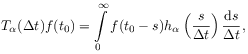
[53.3.1] Consider now the second basic question of Section 2.3.1: How can the fractional order $\alpha$ be observed in experiment or identified from concrete models. [53.3.2] To the best knowledge of this author there exist two examples where this is possible. [53.3.3] Both are related to diffusion processes. [53.3.4] There does not seem to exist an example of a rigorous identification of $\alpha$ from Hamiltonian models, although it has been suggested that such a relation might exist (see [129]).

2.3.4.1 Bochner-Levy Fractional Diffusion

[53.4.1] The term fractional diffusion can refer either to diffusion with a fractional Laplace operator or to diffusion equations with a fractional time derivative. [53.4.2] Fractional diffusion (or Fokker-Planck) equations with a fractional Laplacian may be called Bochner-Levy diffusion. [53.4.3] The identification of the fractional order $\alpha$ in Bochner-Levy diffusion equations has been known for more than five decades [13, 26, 14]. [53.4.4] For a lucid account see also [27]. [53.4.5] The fractional order $\alpha$ in this case is the index of the underlying stable process [13, 27]. [53.4.6] With few exceptions [77] these developments in the nation of mathematics did, for many years, not find much attention or application in the nation of physics although eminent mathematical physicists such as Mark Kac were thoroughly familiar

[page 54, §0] with Bochner-Levy diffusion [65]⁹ (This is a footnote:) ⁹Also, Herrmann Weyl, who pioneered fractional as well as functional calculus and worked on the foundations of physics, seems not to have applied fractional derivatives to problems in physics.. [54.0.1] A possible reason might be the unresolved problem of locality discussed above. [54.0.2] Bochner himself writes ‘‘Whether this (equation) might have physical interpretation, is not known to us’’ [13, p.370].

2.3.4.2 Montroll-Weiss Fractional Diffusion

[54.1.1] Diffusion equations with a fractional time derivative will be called Montroll-Weiss diffusion although fractional time derivatives do not appear in the original paper [87] and the connection was not discovered until 30 years later [60, 46]. [54.1.2] As shown in Section 2.3.3, the locality problem does not arise. [54.1.3] Montroll-Weiss diffusion is expected to be consistent with all fundamental laws of physics. [54.1.4] The fact that the relation between Montroll-Weiss theory and fractional time derivatives was first established in [60, 46] seems to be widely unknown at present, perhaps because this fact is never mentioned in widely read reviews [82] and popular introductions to the subject [112]¹⁰ (This is a footnote:) ¹⁰Note that, contrary to [112, p.51], fractional derivatives are never mentioned in [6]. .

[54.2.1] There exist several versions of diffusion equations with fractional time derivatives, and they differ physically or mathematically from each other [127, 104, 54, 82, 130]. [54.2.2] Of interest here will be the fractional diffusion equation for $f:\mathbb{R}^{d}\times\mathbb{R}_{+}\to\mathbb{R}$

$\mathrm{D}^{{\alpha,1}}_{{0+}}f(\mathbf{r},t)=C\;\Delta f(\mathbf{r},t)$

(2.159)

with a fractional time derivative of order $\alpha$ and type $1$ . [54.2.3] The Laplace operator is $\Delta$ and the fractional diffusion constant is $C$ . [54.2.4] The function $f(\mathbf{r},t)$ is assumed to obey the initial condition $f(\mathbf{r},0+)=f_{0}\delta(\mathbf{r})$ . [54.2.5] Equation (2.159) was introduced in integral form in [104], but the connection with [87] was not given.

[54.3.1] An alternative to eq. (2.159), introduced in [54, 53], is

$\mathrm{D}^{{\alpha,0}}_{{0+}}f(\mathbf{r},t)=C\;\Delta f(\mathbf{r},t)$

(2.160)

with a Riemann-Liouville fractional time derivative $\mathrm{D}^{{\alpha}}_{{0+}}$ of type $0$ . [54.3.2] This equation does not describe diffusion of Montroll-Weiss type [53]. [54.3.3] It has therefore been called ‘‘inconsistent’’ in [81, p.3566]. As emphasized in [53] the choice of $\mathrm{D}^{{\alpha}}_{{0+}}$ in (2.159) is physically and mathematically consistent, but corresponds to a modified initial condition, namely $\mathrm{I}_{{0+}}^{{1-\alpha}}f(\mathbf{r},0+)=f_{0}\delta(\mathbf{r})$ . [54.3.4] Similarly, fractional diffusion equations with time derivative $\mathrm{D}^{{\alpha,\beta}}_{{0+}}$ of order $\alpha$ and type $\beta$ have been investigated in [54]. [54.3.5] For $\alpha=1$ they all reduce to the diffusion equation.

[54.4.1] Before discussing how $\alpha$ arises from an underlying continuous time random walk it is of interest to give an overall comparison of ordinary diffusion with

[page 55, §0] $\alpha=1$ and fractional diffusion of the form (2.159) with $\alpha\neq 1$ . [55.0.1] This is conveniently done using the following table published in [46]. [55.0.2] The first column gives the results for $\alpha=1$ , the second for $0<\alpha<1$ and the third for the limit $\alpha\to 0$ . [55.0.3] The first row compares the infinitesimal generators of time evolution $\mathrm{A}_{\alpha}$ . [55.0.4] The second row gives the fundamental solution $f(\mathbf{k},u)$ in Fourier-Laplace space. [55.0.5] The third row gives $f(\mathbf{k},t)$ and the fourth $f(\mathbf{r},t)$ . [55.0.6] In the fifth and sixth row the asymptotic behaviour is collected for $r^{2}/t^{\alpha}\to 0$ and $r^{2}/t^{\alpha}\to\infty$ .

Table 2.1: Table from [46].


	$\displaystyle\alpha=1$	$\displaystyle 0<\alpha<1$	$\displaystyle\alpha\to 0$

$\displaystyle\mathrm{A}_{\alpha}$	$\displaystyle\frac{\mathrm{d}}{\mathrm{d}t}$	$\displaystyle\widetilde{\mathrm{D}}^{{\alpha}}_{{0+}}$	$\displaystyle\to\mathbf{1}$
$\displaystyle f(\mathbf{k},u)$	$\displaystyle\frac{f_{0}}{u+C\mathbf{k}^{2}}$	$\displaystyle\frac{f_{0}u^{{\alpha-1}}}{u^{\alpha}+C\mathbf{k}^{2}}$	$\displaystyle\to\frac{f_{0}}{u(1+C\mathbf{k}^{2})}$
$\displaystyle f(\mathbf{k},t)$	$\displaystyle f_{0}\mathrm{e}^{{-Ct\mathbf{k}^{2}}}$	$\displaystyle f_{0}\mathrm{E}_{\alpha}\left(-Ct\mathbf{k}^{2}\right)$	$\displaystyle\to\frac{f_{0}}{1+C\mathbf{k}^{2}}$
$\displaystyle f(\mathbf{r},t)$	$\displaystyle\frac{f_{0}\mathrm{e}^{{-\mathbf{r}^{2}/4Ct}}}{(4\pi Ct)^{{-d/2}}}$	$\displaystyle\frac{f_{0}}{(\mathbf{r}^{2}\pi)^{{d/2}}}H^{{d}}_{{\alpha}}\left(\frac{\mathbf{r}^{2}}{4Ct^{\alpha}}\right)$	$\displaystyle\frac{f_{0}\|\mathbf{r}\|^{{1-\frac{d}{2}}}}{\sqrt{C(2\pi)^{{d}}}}K_{{\frac{d-2}{d}}}\left(\frac{\|\mathbf{r}\|}{\sqrt{C}}\right)$
$\displaystyle\frac{\mathbf{r}^{2}}{t^{\alpha}}\to 0$	$\displaystyle t^{{-d/2}}$	$\displaystyle\frac{\|\mathbf{r}\|^{{2-d}}}{t^{\alpha}}$	$\displaystyle\|\mathbf{r}\|^{{(2/d)-(d/2)}}$
$\displaystyle\frac{\mathbf{r}^{2}}{t^{\alpha}}\to\infty$	$\displaystyle\exp\left[-\frac{\mathbf{r}^{2}}{4Ct}\right]$	$\displaystyle\exp\left[-c_{\alpha}\left(\frac{\mathbf{r}^{2}}{4Ct^{\alpha}}\right)^{{\frac{1}{2-\alpha}}}\right]$	$\displaystyle\exp\left(-\frac{\|\mathbf{r}\|}{\sqrt{C}}\right)$

[55.1.1] In the table $\mathrm{E}_{{\alpha,\beta}}(x)$ denotes the generalized Mittag-Leffler function from eq. (2.130), $K_{\nu}(x)$ is the modified Bessel function [1], $d>2$ , $c_{\alpha}=(2-\alpha)\alpha^{{\alpha/(2-\alpha)}}$ and the shorthand

$H^{{d}}_{{\alpha}}\left(x\right)=H^{{20}}_{{12}}\left(x\left|\begin{array}[]{l}{(1,\alpha)}\\ {(d/2,1),(1,1)}\end{array}\right.\right)$

(2.161)

was used for the $H$ -function $H^{{20}}_{{12}}$ . [55.1.2] For information on $H$ -functions see [30, 79, 95, 54].

[page 56, §1] [56.1.1] The results in the table show that the normal diffusion ( $\alpha=1$ ) is slowed down for $0<\alpha<1$ and comes to a complete halt for $\alpha\to 0$ . [56.1.2] For more discussion of the solution see [46].

2.3.4.3 Continuous Time Random Walks

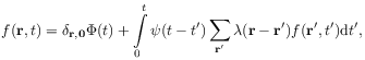
[56.2.1] The fractional diffusion equation (2.159) can be related rigorously to the microscopic model of Montroll-Weiss continuous time random walks (CTRW’s) [87, 64] in the same way as ordinary diffusion is related to random walks [27]. [56.2.2] The fractional order $\alpha$ can be identified and has a physical meaning related to waiting times in the Montroll-Weiss model. [56.2.3] The relation between fractional time derivatives and CTRW’s was first exposed in [60, 46]. [56.2.4] The relation was established in two steps. First, it was shown in [60] that Montroll-Weiss continuous time random walks with a Mittag-Leffler waiting time density are rigorously equivalent to a fractional master equation. [56.2.5] Then, in [46] this underlying random walk model was connected to the fractional diffusion equation (2.159) in the usual asymptotic sense [109] of long times and large distances¹¹ (This is a footnote:) ¹¹This is emphasized in eqs. (1.8) and (2.1) in [46] that are, of course, asymptotic.. [56.2.6] For additional results see also [50, 54, 53, 57]

[56.3.1] The basic integral equation for separable continuous time random walks describes a random walker in continuous time without correlation between its spatial and temporal behaviour. [56.3.2] It reads [87, 88, 118, 39, 64]

$f(\mathbf{r},t)=\delta _{{\mathbf{r},\mathbf{0}}}\Phi(t)+\int\limits _{0}^{t}\psi(t-t^{\prime})\sum _{{\mathbf{r}^{\prime}}}\lambda(\mathbf{r}-\mathbf{r}^{\prime})f(\mathbf{r}^{\prime},t^{\prime})\mathrm{d}t^{\prime},$

(2.162)

where $f(\mathbf{r},t)$ denotes the probability density to find the walker at position $\mathbf{r}\in\mathbb{R}^{d}$ after time $t$ if it started from $\mathbf{r}=\mathbf{0}$ at time $t=0$ . [56.3.3] The function $\lambda(\mathbf{r})$ is the probability for a displacement by $\mathbf{r}$ in each step, and $\psi(t)$ gives the probability density of waiting time intervals between steps. [56.3.4] The transition probabilities obey $\sum _{\mathbf{r}}\lambda(\mathbf{r})=1$ , and $\Phi(t)=1-\int _{0}^{t}\psi(t^{\prime})\mathrm{d}t^{\prime}$ is the survival probability at the initial site.

[56.4.1] The fractional master equation introduced in [60] with inital condition $f(\mathbf{r},0)=\delta _{{\mathbf{r},\mathbf{0}}}$ reads

$\mathrm{D}^{{\alpha,1}}_{{0+}}f(\mathbf{r},t)=\sum _{{\mathbf{r}^{\prime}}}w(\mathbf{r}-\mathbf{r}^{\prime})f(\mathbf{r}^{\prime},t)$

(2.163)

with fractional transition rates $w(\mathbf{r})$ obeying $\sum _{\mathbf{r}}w(\mathbf{r})=0$ . [56.4.2] Note, that eq. (2.162) contains a free function $\psi(t)$ that has no counterpart in eq. (2.163). [56.4.3] The rigorous relation between eq. (2.162) and eq. (2.163), first established in [60], is given by the relation

$\lambda(\mathbf{k})=1+\tau^{\alpha}w(\mathbf{k})$

(2.164)

[page 57, §0] for the Fourier transformed transition rates $w(\mathbf{r})$ and probabilities $\lambda(\mathbf{r})$ , and the choice

$\psi(t)=\frac{t^{{\alpha-1}}}{\tau^{\alpha}}\mathrm{E}_{{\alpha,\alpha}}\left(-\left(\frac{t}{\tau}\right)^{\alpha}\right)$

(2.165)

for the waiting time density, where $\tau>0$ is a characteristic time constant. [57.0.1] With $\mathrm{E}_{{\alpha,\alpha}}(0)=1$ it follows that

$\psi(t)\sim t^{{\alpha-1}}$

(2.166)

for $t\to 0$ . [57.0.2] From $\mathrm{E}_{{\alpha,\alpha}}(x)\sim x^{{-2}}$ for $x\to\infty$ one finds

$\psi(t)\sim t^{{-\alpha-1}}$

(2.167)

for $t\to\infty$ . [57.0.3] For $\alpha=1$ the waiting time density becomes the exponential distribution, and for $\alpha\to 0$ it approaches $1/t$ .

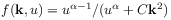
[57.1.1] It had been observed already in the early 1970’s that continuous time random walks are equivalent to generalized master equations [66, 9]. [57.1.2] Similarly, the Fourier-Laplace formula

$f(\mathbf{k},u)=u^{{\alpha-1}}/(u^{\alpha}+C\mathbf{k}^{2})$

(2.168)

for the solution of CTRW’s with algbraic tails of the form (2.167) was well known (see [117, eq.(21), p.402] [110, eq.(23), p.505] [67, eq.(29), p.3083]). [57.1.3] Comparison with row 2 of the table makes the connection between the fractional diffusion equation (2.159) and the CTRW-equation (2.162) evident. [57.1.4] However, this connection with fractional calculus was not made before the appearance of [60, 46]. [57.1.5] In particular, there is no mention of fractional derivatives or fractional calculus in [6].

[57.2.1] The rigorous relation between fractional diffusion and CTRW’s, established in [60, 46] and elaborated in [50, 54, 53, 57], has become a fruitful starting point for subsequent investigations, particularly into fractional Fokker-Planck equations with drift [19, 83, 81, 111, 80, 100, 33, 51, 61, 82, 130, 112].

Acknowledgement: The author thanks Th. Müller and S. Candelaresi for reading the manuscript.

Author:	R. Hilfer
also published in:	Anomalous Transport: Foundations and Applications, Wiley-VCH, Weinheim, page 17-73 (2008), ISBN: 978-3-527-40722-4 Copyright © 2007 R. Hilfer, Stuttgart
first published on:	June 6th, 2007