8 Fractional Time Evolution
[page 214, §1]
[214.1.1] The induced time evolution is obtained from
![]() by iteration.
[214.1.2] According to its definition in eq. (16)
the induced measure preserving transformation
by iteration.
[214.1.2] According to its definition in eq. (16)
the induced measure preserving transformation ![]() acts as a convolution in time,
acts as a convolution in time,
| (17) |
where ![]() is a mixed state on
is a mixed state on ![]() .
[214.1.3] Iterating
.
[214.1.3] Iterating ![]() times gives
times gives
| (18) |
where ![]() is the probability density of the sum
is the probability density of the sum
| (19) |
of ![]() independent
and identically with
independent
and identically with ![]() distributed random
recurrence times
distributed random
recurrence times ![]() .
[214.1.4] Then the long time limit
.
[214.1.4] Then the long time limit ![]() for induced
measure preserving transformations on subsets of
small measure is generally governed by
well known local limit theorems for convolutions
[42, 43, 44, 45].
[214.1.5] Application to the case at hand yields
the following fundamental theorem of fractional
dynamics [1, 21]
for induced
measure preserving transformations on subsets of
small measure is generally governed by
well known local limit theorems for convolutions
[42, 43, 44, 45].
[214.1.5] Application to the case at hand yields
the following fundamental theorem of fractional
dynamics [1, 21]
Theorem 8.1.
Assume that ![]() is maximal in the sense that there is no larger
is maximal in the sense that there is no larger
![]() for which all recurrence
times lie in
for which all recurrence
times lie in ![]() .
[214.1.6] Then the following conditions are equivalent:
.
[214.1.6] Then the following conditions are equivalent:
[214.1.7] Either
 or there exists a number
  such that
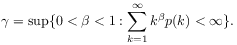
(20) [214.1.8] There exist constants
 and
and  such that
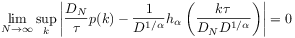
(21) where
 , if ,
and
, if ,
and  otherwise.
[214.1.9] The function
otherwise.
[214.1.9] The function  vanishes for
  , and is
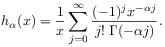
(22) for
 .
.
[page 215, §0]
[215.0.1] If the limit exists, and is nondegenerate, i.e. ![]() , then
the rescaling constants
, then
the rescaling constants ![]() have the form
have the form
| (23) |
where ![]() is a slowly varying function [46], i.e.
is a slowly varying function [46], i.e.
| (24) |
for all ![]() .
.
[215.1.1] The theorem shows that
| (25) |
holds for sufficiently large ![]() .
[215.1.2] The asymptotic behaviour of the iterated
induced measure preserving transformation
.
[215.1.2] The asymptotic behaviour of the iterated
induced measure preserving transformation ![]() for
for ![]() allows to remove the discretization,
and to find the induced continuous time evolution on
subsets
allows to remove the discretization,
and to find the induced continuous time evolution on
subsets ![]() .
[215.1.3] First, the definition eq. (15)
is extended from the arithmetic progression
.
[215.1.3] First, the definition eq. (15)
is extended from the arithmetic progression ![]() to
to ![]() by linear interpolation.
[215.1.4] Let
by linear interpolation.
[215.1.4] Let ![]() denote the extended measure
defined for
denote the extended measure
defined for ![]() .
[215.1.5] Using eq. (11) and setting
.
[215.1.5] Using eq. (11) and setting
| (26) |
the summation in eq. (18) can
be approximated for sufficently large ![]() by an integral.
[215.1.6] Then
by an integral.
[215.1.6] Then ![]() ,
where
,
where
![{\rule[-2.0pt]{0.0pt}{10.0pt}_{{{G}}}\! T}_{\alpha}^{t}\widetilde{\varrho}({\dot{s}})=\int\limits _{0}^{\infty}\widetilde{\varrho}({\dot{s}}-{\dot{t}})h_{\alpha}\left(\frac{{\dot{t}}}{t}\right)\frac{\mathrm{d}{\dot{t}}}{t}](mi/mi141.png) |
(27) |
is the induced continuous time evolution.[215.1.7]
![]() is also called fractional time evolution.
[215.1.8] Laplace tranformation shows that
is also called fractional time evolution.
[215.1.8] Laplace tranformation shows that ![]() fulfills eq. (5).
[215.1.9] It is an example of subordination of semigroups
[47, 33, 7, 48].
[215.1.10] Indeed
fulfills eq. (5).
[215.1.9] It is an example of subordination of semigroups
[47, 33, 7, 48].
[215.1.10] Indeed
![{\rule[-2.0pt]{0.0pt}{10.0pt}_{{{G}}}\! T}_{\alpha}^{t}=\frac{1}{t}\int\limits _{0}^{\infty}T^{{\dot{t}}}h_{\alpha}\left(\frac{{\dot{t}}}{t}\right)\mathrm{d}{\dot{t}}](mi/mi140.png) |
(28) |
where ![]() denotes right translations
on the interpolated measure.
[215.1.11] Because
denotes right translations
on the interpolated measure.
[215.1.11] Because ![]() and
and ![]() ,
eq. (26) implies
,
eq. (26) implies ![]() .
[215.1.12] As remarked in the introduction,
the induced time evolution
is in general not a translation (group or semigroup), but
a convolution semigroup.
[215.1.13] The fundamental classification parameter
.
[215.1.12] As remarked in the introduction,
the induced time evolution
is in general not a translation (group or semigroup), but
a convolution semigroup.
[215.1.13] The fundamental classification parameter
| (29) |
[page 216, §0]
depends not only on the dynamical rule ![]() and the subset
and the subset ![]() , but also on the discretization time
step
, but also on the discretization time
step ![]() , i.e. on the time scale of interest.
, i.e. on the time scale of interest.
