11 Experimental Evidence
[218.2.1] If fractional time evolutions from eq. (27)
with ![]() must be expected on general grounds, then they
should be observable in experiment.
[218.2.2] Numerous experimental examples of anomalous dynamics or strange
kinetics have been identified (see [17, 18, 19, 20]
and the present volume for reviews).
[218.2.3] Here the example of dielectric
must be expected on general grounds, then they
should be observable in experiment.
[218.2.2] Numerous experimental examples of anomalous dynamics or strange
kinetics have been identified (see [17, 18, 19, 20]
and the present volume for reviews).
[218.2.3] Here the example of dielectric ![]() -relaxation in glasses
is briefly discussed[53, 54], because it provides
experimental data over up to 19 decades in time [55],
and because the explanation of its excess wing has been
a matter of debate.
-relaxation in glasses
is briefly discussed[53, 54], because it provides
experimental data over up to 19 decades in time [55],
and because the explanation of its excess wing has been
a matter of debate.
[218.3.1] For every induced time evolution on ![]() with time scale
with time scale ![]() and fractional order
and fractional order ![]()
| (36) |
holds generally with ![]() .
[218.3.2] A physical system typically shows different
physical phenomena on different time scales
.
[218.3.2] A physical system typically shows different
physical phenomena on different time scales ![]() .
[218.3.3] In [53, 54] it was assumed that
the second factor in eq. (36) becomes
approximately fractional in the sense that
.
[218.3.3] In [53, 54] it was assumed that
the second factor in eq. (36) becomes
approximately fractional in the sense that
| (37) |
holds in the weak* or strong topology with
| (38) |
[218.3.4] The resulting composite time evolution
![]() was studied in [53, 54]
for the case
was studied in [53, 54]
for the case ![]() .
[218.3.5] Rescaling this composite operator as in the case of Debye relaxation
and computing the infinitesimal generator yields
the fractional differential equation [53, 54]
.
[218.3.5] Rescaling this composite operator as in the case of Debye relaxation
and computing the infinitesimal generator yields
the fractional differential equation [53, 54]
| (39) |
[page 219, §0]
with ![]() from eq. (33) and inital value
from eq. (33) and inital value ![]() .
[219.0.1] Its solution is
.
[219.0.1] Its solution is
| (40) |
where
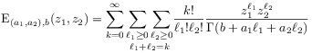 |
(41) |
with ![]() and
and ![]() is the binomial Mittag-Leffler function [61].
is the binomial Mittag-Leffler function [61].
[page 220, §1]
[220.1.1] The complex frequency dependent
susceptibility is obtained from the
the normalized relaxation
function as
![]() where
where ![]() is the Laplace transform
of
is the Laplace transform
of ![]() and
and ![]() is the imaginary
circular frequency [54, p. 402, eq.(18)].
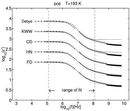
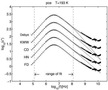
[220.1.2] The real part of the complex dielectric susceptibility for
propylene carbonate at temperature
is the imaginary
circular frequency [54, p. 402, eq.(18)].
[220.1.2] The real part of the complex dielectric susceptibility for
propylene carbonate at temperature ![]() K is plotted
in Figure 1, its imaginary part in
Figure 2.
[220.1.3] These figures are taken from [53].
[220.1.4] Crosses represent experimental data.
[220.1.5] Different fit functions are shifted
by half a decade for better visibility.
[220.1.6] The range over which the data were fitted
is indicated by two
dashed vertical lines.
[page 221, §0]
[221.0.1] The curve labelled FD (fractional dynamics)
is the susceptibility corresponding to the
relaxation function in eq. (40)
It reproduces the high frequency wing
even outside the range of its fit.
[221.0.2] This is not the case for the other four curves
curves, labelled Debye,
KWW, CD and HN.
They correspond to four
popular fit functions for dielectric relaxation
[55, 62].
[221.0.3] The curve Debye corresponds to a simple exponential
function, KWW (Kohlrausch-Williams-Watts)
is a stretched exponential relaxation function.
[221.0.4] The relaxation functions for the two remaining cases,
CD (Cole-Davison) and HN
(Havriliak-Negami) were given for the first time in [58, 60].
K is plotted
in Figure 1, its imaginary part in
Figure 2.
[220.1.3] These figures are taken from [53].
[220.1.4] Crosses represent experimental data.
[220.1.5] Different fit functions are shifted
by half a decade for better visibility.
[220.1.6] The range over which the data were fitted
is indicated by two
dashed vertical lines.
[page 221, §0]
[221.0.1] The curve labelled FD (fractional dynamics)
is the susceptibility corresponding to the
relaxation function in eq. (40)
It reproduces the high frequency wing
even outside the range of its fit.
[221.0.2] This is not the case for the other four curves
curves, labelled Debye,
KWW, CD and HN.
They correspond to four
popular fit functions for dielectric relaxation
[55, 62].
[221.0.3] The curve Debye corresponds to a simple exponential
function, KWW (Kohlrausch-Williams-Watts)
is a stretched exponential relaxation function.
[221.0.4] The relaxation functions for the two remaining cases,
CD (Cole-Davison) and HN
(Havriliak-Negami) were given for the first time in [58, 60].
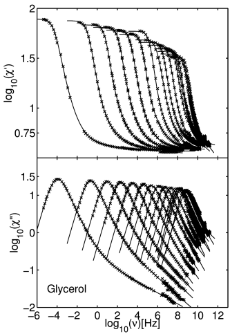
[221.1.1] Figure 3 from [54]
shows the real and imaginary part of the
dielectric susceptibility for glycerol as
its temperature varies over the
glass transition range from ![]() K to
K to ![]() K.
[221.1.2] The fits are based on a trinomial fractional relaxation
function as detailed in [54, 61].
K.
[221.1.2] The fits are based on a trinomial fractional relaxation
function as detailed in [54, 61].