2 Classical relaxation models
[1283.4.1] The Debye relaxation model describes the electric relaxation of
dipoles after switching an applied electric field [21].
[1283.4.2] The normalized relaxation function ![]() ,
which corresponds to the polarization,
obeys the Debye law
,
which corresponds to the polarization,
obeys the Debye law
| (1) |
[page 1284, §0]
with the relaxation time ![]() and initial condition
and initial condition ![]() .
[1284.0.1] The response function, i.e. the dynamical dielectric susceptibility,
.
[1284.0.1] The response function, i.e. the dynamical dielectric susceptibility, ![]() is related to the relaxation function via [17]
is related to the relaxation function via [17]
| (2) |
[1284.0.2] In the following discussions we focus on Laplace transformed quantities.
[1284.0.3] We use the Laplace transformation of ![]()
| (3) |
where ![]() and
and ![]() is the frequency.
[1284.0.4] Rewriting equation (2) in frequency space and
using
is the frequency.
[1284.0.4] Rewriting equation (2) in frequency space and
using ![]() leads to
leads to
| (4) |
the well known Debye susceptibility.
[1284.0.5] In experiments one measures not the normalized quantity ![]() ,
but instead
,
but instead
| (5) |
where ![]() and
and ![]() are the dynamical
susceptibilities at low, respectively high frequencies.
are the dynamical
susceptibilities at low, respectively high frequencies.
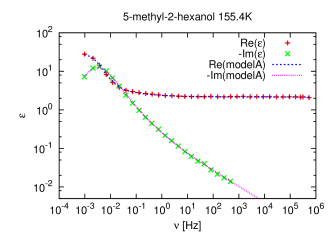
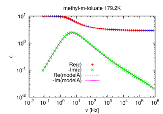
[1284.1.1] The Debye model is not able to describe the experimental data well,
because experimental relaxation peaks are broader and asymmetric.
[1284.1.2] For this reason other fitting functions were proposed such as the
Cole-Cole [22], Cole-Davidson [23]
and Havriliak-Negami [16] expressions.
[1284.1.3] Their normalized forms have typically 2 or 3 parameters
(see table 1) and
they were introduced purely phenomenologically to fit the data.
[1284.1.4] This can be considered as a drawback.
[1284.1.5] These functions with three parameters
are able to fit the data over a range of at most ![]() decades (Havriliak-Negami).
[1284.1.6] To fit a broader frequency range
several functions are commonly added.
[1284.1.7] A combination of one Havriliak-Negami expression
plus one Cole-Cole form results in 6 fit parameters.
decades (Havriliak-Negami).
[1284.1.6] To fit a broader frequency range
several functions are commonly added.
[1284.1.7] A combination of one Havriliak-Negami expression
plus one Cole-Cole form results in 6 fit parameters.
|
functional
form |
number of parameters |
|
|---|---|---|
| Cole-Cole | 2 | |
| Cole-Davidson | 2 | |
| Havriliak-Negami | 3 |
 |
 |
 |
 |
