V.A Effective Transport Coefficients

V.A.1 Definition

A large number of transport and relaxation processes in porous media are governed by the diordered Laplace equation (4.2) with variable coefficients ${\bf C}({\bf r})$ for a scalar field $P({\bf r})$

$\nabla^{T}\cdot({\bf C}({\bf r})\nabla P({\bf r}))=0$

(5.1)

within the sample region $\mathbb{S}=\mathbb{P}\cup\mathbb{M}$ . This “equation of motion” for $P$ must be supplemented with suitable boundary conditions on the sample boundary $\partial\mathbb{S}$ , and, if ${\bf C}({\bf r})$ is discontinuous across $\partial\mathbb{P}$ , also on the internal boundary $\partial\mathbb{P}$ . Introducing the vector field ${\bf v}({\bf r})$ the equation (5.1) may be rewritten as

$\displaystyle{\bf v}({\bf r})$	$\displaystyle=$	$\displaystyle-{\bf C}({\bf r})\mbox{\boldmath$\nabla$}P({\bf r})$		(5.2)
$\displaystyle\mbox{\boldmath$\nabla$}^{T}\cdot{\bf v}({\bf r})$	$\displaystyle=$	$\displaystyle 0.$

These equations can be used as the microscopic starting point although, as shown below in section V.C.3 for the case of fluid flow, they may hold only in a macroscopic limit starting from a different underlying microscopic description. Equations (5.1) or (5.2) appear in many transport and relaxation problems for porous and heterogeneous media. For Darcy flow in porous media $P$ is the pressure, ${\bf C}={\bf K}/\eta$ is the quotient of absolute hydraulic permeability and fluid viscosity, and ${\bf v}$ is the fluid velocity field. For dielectric relaxation $P$ becomes the electrostatic potential, ${\bf v}$ becomes the dielectric displacement and ${\bf C}$ becomes the dielectric permittivity tensor. In diffusion or dispersion problems $P$ is the concentration field, ${\bf v}$ corresponds to the diffusion flux and ${\bf C}$ becomes the diffusivity. Table III summarizes the translation of $P,{\bf v}$ and ${\bf C}$ into various problems.

Table III: Quantities corresponding to $P,{\bf v}$ and ${\bf C}$ in 5.2 for different transport and relaxation problems in porous media.

Problem Type	$P$	${\bf v}$	${\bf C}$
fluid flow	pressure	velocity	$\frac{\rm permability}{\rm viscosity}$
electrical conduction	voltage	current	conductivity
dielectric relaxation	potential	displacement	dielectric permittivity
diffusion (dispersion)	concentration	particle flux	diffusion constant

For a homogeneous and isotropic medium the transport coefficients ${\bf C}({\bf r})=C{\bf 1}$ , where ${\bf 1}$ denotes the identity, are independent of ${\bf r}$ , and (5.1) reduces to a Laplace equation for the field $P$ . For a random medium the transport coefficients are random functions of ${\bf r}$ and the solutions $P({\bf r})$ and ${\bf v}({\bf r})$ depend on the realization of ${\bf C}({\bf r})$ . The averaged solutions $\left\langle P({\bf r})\right\rangle$ and $\left\langle{\bf v}({\bf r})\right\rangle$ are therefore of primary interest. The tensor of effective transport coefficients is $\overline{{\bf C}}$ defined as

$\left\langle{\bf v}({\bf r})\right\rangle=-\overline{{\bf C}}\mbox{\boldmath$\nabla$}\left\langle P({\bf r})\right\rangle,$

(5.3)

and it provides a relation between the average fields. The ensemble averages $\left\langle f({\bf r})\right\rangle$ in the definition can be replaced with spatial averages defined by

$\overline{f}=\frac{1}{V(\mathbb{S})}\int f({\bf r})\chi\rule[-4.3pt]{0.0pt}{8.6pt}_{{\mathbb{S}}}({\bf r})d^{3}{\bf r}$

(5.4)

where $f$ stands for $P$ or ${\bf v}$ . Both the ensemble and the spatial average depend on the averaging region $\mathbb{S}$ , and a residual variation of $\overline{f}$ or $\left\langle f\right\rangle$ is possible on scales larger than the size of $\mathbb{S}$ . In the following it will always be assumed that $\overline{f}=\left\langle f\right\rangle$ if $\mathbb{S}$ is sufficiently large. The ensemble average notation will be preferred because it is notationally more convenient.

The purpose of introducing effective macroscopic transport coefficients is to replace the heterogeneous medium described by ${\bf C}({\bf r})$ with an equivalent homogeneous medium described by $\overline{{\bf C}}$ . If $\overline{{\bf C}}$ is known then all the knowledge accumulated for the homogeneous problem can be utilized immediately, and e.g. the average field ${\bf v}$ can be obtained simply from solving a Laplace equation for $P$ .

V.A.2 Discretization and Networks

If the function ${\bf C}({\bf r})$ is known then equation (5.1) can be solved to any desired accuracy using standard finite difference approximation schemes. To this end the sample space $\mathbb{S}$ of linear extension $\mathcal{L}$ is partitioned into cubes $\mathbb{K}_{j}$ . The cubes are centered on the sites ${\bf r}_{i}$ of a simple cubic lattice with lattice spacing $L$ . Other lattices may also be employed. The lengths $L$ and $\mathcal{L}$ obey $L\ll\mathcal{L}$ . The total numer of cubes is $N=(\mathcal{L}/L)^{d}$ .

For a stationary and isotropic medium with ${\bf C}({\bf r})=c({\bf r}){\bf 1}$ the discretization of equation (5.1) gives a system of linear equations for the pressure variables at the cube centers $P_{i}=P({\bf r}_{i})$

$\sum _{j}c_{{ij}}(P_{i}-P_{j})=0$

(5.5)

for cubes ${\bf r}_{i}$ not located at the sample boundary. The boundary conditions at the sample boundary give rise to a nonvanishing right hand side of the linear system if ${\bf r}_{i}$ is the center of a cube located close to $\partial\mathbb{S}$ . The local transport coefficients $c_{{ij}}$ are given as

$c_{{ij}}(L)=c\left(({\bf r}_{i}+{\bf r}_{j})/2\right)$

(5.6)

if ${\bf r}_{i}$ and ${\bf r}_{j}$ are nearest neighbours. If ${\bf r}_{i}$ and ${\bf r}_{j}$ are not nearest neighbours the local coefficient vanishes, $c_{{ij}}=0$ . Because the location of the cube centers ${\bf r}_{i}$ depends on the resolution $L$ the coefficients $c_{{ij}}$ in the network equations depend on $L$ and on the shape of the measurement cells $\mathbb{K}_{i}$ .

The numerical solution of the discretized equations (5.5) can be obtained by many methods including relaxation, successive overrelaxation or conjugate gradient schemes, transfer matrix calculations, series expansions or recursion methods [263, 264, 265, 266, 248, 267, 40]. If the function $c({\bf r})$ is known then the solution to (5.1) is recovered in the limit $L\rightarrow 0$ to any desired accuracy. Within a certain class of lattices the limit is known to be independent of the choice of the approximating discrete lattice. To actually perform this limit, however, the function $c({\bf r})$ must be known to arbitrary accuracy.

In most experimental and practical problems the function $c({\bf r})$ is either completely unknown or not known to arbitrary accuracy. Therefore it is necessary to have a theory for the local transport coefficients $c_{{ij}}(L)$ as a function of the resolution $L$ of the discretization. At present the only resolution dependent theories seem to be local porosity theory [168, 169, 170, 171, 172, 173, 174, 175] and homogenization theory [268, 269, 270, 38, 271] which will be discussed in more detail below. The basic idea of local porosity theory is to use the local geometry distributions defined in section III.A.5 and to express the local transport coefficients in terms of the geometrical quantities characterizing the local geometry. The basic idea of homogenization theory is a double scale asymptotic expansion in the small parameter $L/\mathcal{L}$ .

The discretized equations (5.5) are network equations. This explains the great importance and popularity of network models. In the more conventional network models [220, 221, 222, 223, 225, 187, 226, 227, 228, 229, 230, 155, 157, 231, 232, 233] the resolution dependence is neglected altogether. Instead one assumes a specific model for the local transport coefficients $c_{{ij}}$ such that the global geometric characteristics (porosity etc.) are reproduced by the model. Three immediate problems arise from this assumption:

The connection with the underlying local geometry is lost, although the local value of the transport property depends on it.
In the absence of an independent measurement of the local transport coefficients they become free fit parameters. Popular stochastic network models assume lognormal or binary distributions for the local transport coefficients.
Without a model for the local geometry an independent experimental or calculational determination of the local transport coefficients for one transport problem (say fluid flow) cannot be used for another transport problem (say diffusion) although the equations of motion (5.1) have the same mathematical form for both cases.

All of these problems are alleviated in local porosity theory or homogenization theory which attempt to keep the connection with the underlying local geometry.

V.A.3 Simple Expressions for Effective Transport Coefficients

While a numerical solution of the network equations (5.5) is of great practical interest, its value for a scientific understanding of heterogeneous media is limited. Analytical expressions, be they exact or approximate, are better suited for developing the theory because they allow to extract the general modelindependent aspects. Unfortunately only very few exact analytical results are available [272, 273, 274, 275]. The one dimensional case can be solved exactly by a change of variable. The exact result is the harmonic average

$\overline{c}=\left\langle c^{{-1}}\right\rangle^{{-1}}$

(5.7)

where the average denotes either an average with respect to $w(c)$ , the probability density of local transport coefficients, or a spatial average as defined in (5.4). In two dimensions the geometric average

$\overline{c}=\exp\left\langle\log c\right\rangle=\frac{\left\langle c\right\rangle^{{1/2}}}{\left\langle c^{{-1}}\right\rangle^{{1/2}}}$

(5.8)

has been obtained exactly using duality in harmonic function theory [272] if the microsctructure is homogeneous, isotropic and symmetric. It was later rederived under less stringent conditions [273] and generalized to isomorphisms between associated microstructures [274].

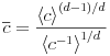
Most analytical expressions for effective transport properties are approximate. In general dimensions approximation formulae such as [276, 277, 275]

$\overline{c}=\frac{\left\langle c\right\rangle^{{(d-1)/d}}}{\left\langle c^{{-1}}\right\rangle^{{1/d}}}$

(5.9)

or [278, 279]

$\overline{c}=\left\langle c^{{(1-2/d)}}\right\rangle^{{1/(1-2/d)}}$

(5.10)

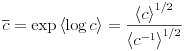
have been suggested which reduce to the exact results for $d=1$ and $d=\infty$ . Various mean field theories also provide approximate estimates for the effective permeabilities. The simplest mean field theory

$\overline{c}=\left\langle c\right\rangle$

(5.11)

is obtained from equations (5.9) or (5.10) by letting $d\rightarrow\infty$ . Another very important approximation is the selfconsistent effective medium approximation which reads

$\left\langle\frac{c-\overline{c}}{c+(d-1)\overline{c}}\right\rangle=0$

(5.12)

for a $d$ -dimensional hypercubic lattice. For other regular lattices the factor $d-1$ in the denominator has to be replaced with $(z/2)-1$ where $z$ is the coordination number of the lattice. Note that for $d=1$ and $d\rightarrow\infty$ the effective medium approximation reproduces the exact result.

To distinguish the quality of these approximations it is instructive to consider a probability density $w(c)$ of local transport coefficients which has a finite fraction $p=1-\lim _{{\varepsilon\rightarrow 0}}\int _{0}^{\varepsilon}w(c)dc$ of blocking bonds. In dimension $d>1$ this implies the existence of a percolation threshold $0<p_{c}<1$ below which $\overline{c}=0$ vanishes identically (see Table II for values of $p_{c}$ ). Among the expressions (5.7) through (5.12) only the effective medium approximation (5.12) is able to predict the existence of a transition. The predicted critical value $p_{c}=1/d$ , however, is not exact as seen by comparison with Table II.

Another method for calculating the effective or transport coefficient $\overline{c}$ will be discussed in homogenization theory in section V.C.4. The resulting expression appears in equation (5.87) if one sets ${\bf K}=c{\bf 1}$ . It is given as as a correction to the simplest mean field expression (5.11). The correction involves the fundamental solution of the local transport problem (5.88). In practice the use of (5.87) is restricted to simple periodic microstructures [268, 280]. If the microsctructure is periodic it suffices to obtain the fundamental solutions within the basic period, and to extend the average in (5.87) over that period. If the microstructure is not periodic then the solution of (5.88) and averaging in (5.87) quickly become as impractical as solving the original problem, because $c({\bf r})$ is then unknown.

Author:	R. Hilfer
originally published in:	Advances in Chemical Physics 92, 299-424 (1996)
originally submitted:	May 9th, 1995