VII Amplitude ratios
[74.1.2.1] This section discusses universal amplitudes such as those
defined in (1.6) and their ratios.
[74.1.2.2] In numerical
simulations of critical phenomena amplitude ratios such as
(1.7) are used routinely to extract critical parameters
![]() and exponents from simulations of finite systems.
[74.1.2.3] It is then of interest to analyze finite size amplitude
ratios within the present framework.
and exponents from simulations of finite systems.
[74.1.2.3] It is then of interest to analyze finite size amplitude
ratios within the present framework.
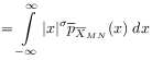
[74.1.3.1] The absolute moment of order ![]() for the ensemble averages
of
for the ensemble averages
of ![]() in a finite and noncritical system is found from
equations (4.4) and (3.16) as
in a finite and noncritical system is found from
equations (4.4) and (3.16) as
 |
(7.1) | ||
| (7.2) |
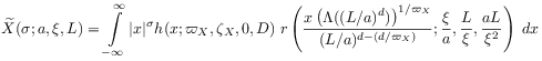
where the amplitude ![]() of the finite, discrete and
noncritical system is given as
of the finite, discrete and
noncritical system is given as
 |
(7.3) |
and the function ![]() is defined from
equation (4.7) by replacing
is defined from
equation (4.7) by replacing ![]() with
with ![]() and extracting
a factor
and extracting
a factor ![]() .
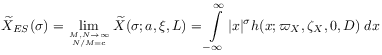
[74.2.0.1] In the ensemble limit one obtains from this and (3.17) the result
.
[74.2.0.1] In the ensemble limit one obtains from this and (3.17) the result
 |
(7.4) |
for the critical ensemble scaling amplitude of order ![]() in an
infinite system.
[74.2.0.2] The subscript is again a reminder for the ensemble
scaling limit.
[74.2.0.3] The integral in (7.4) can be evaluated for
in an
infinite system.
[74.2.0.2] The subscript is again a reminder for the ensemble
scaling limit.
[74.2.0.3] The integral in (7.4) can be evaluated for ![]() as
as
| (7.5) |
which is valid for ![]() and
and
![]() .
[74.2.0.4] A derivaton of this result is given in Appendix B.
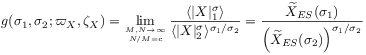
[74.2.0.5] This allows to calculate the general moment ratios
.
[74.2.0.4] A derivaton of this result is given in Appendix B.
[74.2.0.5] This allows to calculate the general moment ratios
 |
(7.6) |
with ![]() in the ensemble limit.
[74.2.0.6] Figure 6 shows a twodimensional plot of the ratio
in the ensemble limit.
[74.2.0.6] Figure 6 shows a twodimensional plot of the ratio
![]() .
.

[74.2.1.1] If equation (7.5) is used to analytically continue
![]() beyond the regime
beyond the regime ![]() the traditional
fourth order cumulant
the traditional
fourth order cumulant ![]() for the order
parameter is found to exhibit special problems if
for the order
parameter is found to exhibit special problems if ![]() .
[74.2.1.2] This is mainly due to the presence of the factor
.
[74.2.1.2] This is mainly due to the presence of the factor ![]() in (7.5).
[74.2.1.3] The divergence must somehow become absorbed by the
cutoff factor
in (7.5).
[74.2.1.3] The divergence must somehow become absorbed by the
cutoff factor ![]() in the finite size scaling limit.
[74.2.1.4] Assuming that this is indeed the case it is then of interest
to consider the quantity
in the finite size scaling limit.
[74.2.1.4] Assuming that this is indeed the case it is then of interest
to consider the quantity
| (7.7) |
[page 75, §0] in the finite size scaling limit assuming that it exists. [75.1.0.1] Then the traditional finite size cumulant becomes
 |
(7.8) |
[75.1.0.2] The interest in this formal expression is that it is still singular.
[75.1.0.3] Within the domain ![]() it
has simple poles along the lines
it
has simple poles along the lines
![\begin{array}[]{l}\varpi _{X}=\dfrac{4}{3}\\
\varpi _{X}=\dfrac{4\zeta _{X}}{2\zeta _{X}\pm 1}\end{array}](mi/mi359.png) |
(7.9) |
and zeros along the lines
![\begin{array}[]{l}\varpi _{X}=\dfrac{8\zeta _{X}}{4\zeta _{X}\pm 1}\\
\varpi _{X}=\dfrac{8\zeta _{X}}{4\zeta _{X}\pm 3}.\end{array}](mi/mi360.png) |
(7.10) |
[75.1.0.4] For the traditionally studied order parameter cumulant, i.e.
setting ![]() , the pole at
, the pole at ![]() implies a divergence whenever
implies a divergence whenever
![]() , i.e. in mean field theory.
[75.1.0.5] This result is consistent with
the divergence
, i.e. in mean field theory.
[75.1.0.5] This result is consistent with
the divergence ![]() found in conformal
field theory [17].
[75.1.0.6] Note that the points
found in conformal
field theory [17].
[75.1.0.6] Note that the points ![]() along the singular mean field line
along the singular mean field line ![]() are intersection
points with a line of zeros.
are intersection
points with a line of zeros.
[75.1.1.1] Irrespective of these problems it is of interest to estimate
values for the traditional order parameter cumulant ratio
![]() because much previous work has focussed on it.
[75.1.1.2] Within the present approach this is possible from the knowledge
of the scaling functions if it is assumed that the identification
of
because much previous work has focussed on it.
[75.1.1.2] Within the present approach this is possible from the knowledge
of the scaling functions if it is assumed that the identification
of ![]() with periodic boundary conditions holds generally.
[75.1.1.3] If the scaling functions with
with periodic boundary conditions holds generally.
[75.1.1.3] If the scaling functions with ![]() in Figures 2 through 4
are simply truncated
sharply at
in Figures 2 through 4
are simply truncated
sharply at ![]() ,
and subseqently rescaled to unit norm and variance, the order
parameter cumulant
,
and subseqently rescaled to unit norm and variance, the order
parameter cumulant ![]() may be calculated as usual,
and it will depend upon the nonuniversal cutoff at
may be calculated as usual,
and it will depend upon the nonuniversal cutoff at ![]() .
[75.2.0.1] The results of such a cutoff procedure are displayed in Figure 7
for the cases
.
[75.2.0.1] The results of such a cutoff procedure are displayed in Figure 7
for the cases ![]() .
[75.2.0.2] It is seen that the cumulant is distinctly cutoff dependent.
[75.2.0.3] Note that all curves appear
to diverge as the cutoff increases.
.
[75.2.0.2] It is seen that the cumulant is distinctly cutoff dependent.
[75.2.0.3] Note that all curves appear
to diverge as the cutoff increases.

[75.2.0.4] For the cases ![]() and
and ![]() some structure appears
between
some structure appears
between ![]() and
and ![]() corresponding to the strong curvature
in this region seen in Figures 2 and 3.
[75.2.0.5] For the
corresponding to the strong curvature
in this region seen in Figures 2 and 3.
[75.2.0.5] For the ![]() -Ising case the
curve is flat up to about twice the maximal value
-Ising case the
curve is flat up to about twice the maximal value ![]() for the
simulations of Bruce and coworkers [43, 45].
[75.2.0.6] Figure 5 provides a possible explanation for the poor
agreement between the value
for the
simulations of Bruce and coworkers [43, 45].
[75.2.0.6] Figure 5 provides a possible explanation for the poor
agreement between the value ![]() observed in simulations of the fivedimensional Ising model
[11, 46] and the mean field calculation
observed in simulations of the fivedimensional Ising model
[11, 46] and the mean field calculation
![]() from [15].
[75.2.0.7] The simulation result
is indicated as the solid arrow, the analytical result as the
dashed arrow pointing to the curve
from [15].
[75.2.0.7] The simulation result
is indicated as the solid arrow, the analytical result as the
dashed arrow pointing to the curve ![]() .
[75.2.0.8] The small difference
in the cutoff
.
[75.2.0.8] The small difference
in the cutoff ![]() corresponding to these values suggests that
the discrepancy may result from different nonuniversal (but most
likely smooth) cutoffs in the two estimates.
corresponding to these values suggests that
the discrepancy may result from different nonuniversal (but most
likely smooth) cutoffs in the two estimates.
[75.2.1.1] Finally, the fact that the value of the universal shape parameter ![]() appears to be related to the choice of bondary conditions suggests a
method of constructing critical amplitude ratios which do not depend on
boundary conditions, or other factors influencing
appears to be related to the choice of bondary conditions suggests a
method of constructing critical amplitude ratios which do not depend on
boundary conditions, or other factors influencing ![]() .
[75.2.1.2] The
basic idea is to use the difference of two independent observations
of ensemble averages or sums.
[75.2.1.3] Let
.
[75.2.1.2] The
basic idea is to use the difference of two independent observations
of ensemble averages or sums.
[75.2.1.3] Let ![]() and
and ![]() be
two independent measurements and
be
two independent measurements and ![]() their difference.
[75.2.1.4] The limiting distribution function
their difference.
[75.2.1.4] The limiting distribution function
![]() for
for ![]() and
and ![]() at criticality
is given in equation (4.2).
[75.2.1.5] Then the difference
at criticality
is given in equation (4.2).
[75.2.1.5] Then the difference
![]() has the distribution function
has the distribution function
| (7.11) |
[page 76, §0]
in which the width is doubled, but ![]() has disappeared.
[76.1.0.1] The
fractional difference moment ratio
has disappeared.
[76.1.0.1] The
fractional difference moment ratio ![]() is formed analogously to the moment ratio
is formed analogously to the moment ratio ![]() as
as
| (7.12) |
and it has a universal value depending only on the scaling
dimension of ![]() as long as
as long as ![]() .
[76.1.0.2] If the scaling dimension is universal then the fractional
difference moment ratio is independent of boundary
conditions.
[76.1.0.3] Plotting
.
[76.1.0.2] If the scaling dimension is universal then the fractional
difference moment ratio is independent of boundary
conditions.
[76.1.0.3] Plotting ![]() as
a function of length
scale and temperature should then allow
to extract the critical exponent.
as
a function of length
scale and temperature should then allow
to extract the critical exponent.
