II Scaling limits
[64.2.3.1] The finite size scaling limit ![]() with
with ![]() constant
is a special kind of field theoretical scaling limit.
[64.2.3.2] A fieldtheoretic
scaling limit involves three different limits: 1. The thermodynamic
limit
constant
is a special kind of field theoretical scaling limit.
[64.2.3.2] A fieldtheoretic
scaling limit involves three different limits: 1. The thermodynamic
limit ![]() in which the system size becomes large, 2. the continuum
limit
in which the system size becomes large, 2. the continuum
limit ![]() in which a microscopic length becomes small, and 3.
the critical
[page 65, §0]
limit
in which a microscopic length becomes small, and 3.
the critical
[page 65, §0]
limit ![]() in which the correlation length of
a particular observable (scaling field) diverges.
in which the correlation length of
a particular observable (scaling field) diverges.
[65.1.1.1] This section discusses the recently introduced ensemble limit [20, 21, 22, 23] as a novel kind of field theoretic scaling limit, and relates it to traditional limiting procedures.
II.A Discretization in field theory
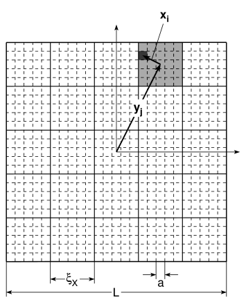
[65.1.2.1] Consider a macroscopic classical continuous system within a cubic
subset of ![]() with volume
with volume ![]() and linear extension
and linear extension ![]() .
[65.1.2.2] The
finite macroscopic volume
.
[65.1.2.2] The
finite macroscopic volume ![]() is partitioned into
is partitioned into ![]() mesoscopic
cubic blocks of linear size
mesoscopic
cubic blocks of linear size ![]() .
[65.1.2.3] The coordinate of the center of
each block is denoted by
.
[65.1.2.3] The coordinate of the center of
each block is denoted by ![]() .
[65.1.2.4] Each block is further
partitioned into
.
[65.1.2.4] Each block is further
partitioned into ![]() microscopic cells of linear size
microscopic cells of linear size ![]() whose
coordinates with respect to the center of the block are denoted as
whose
coordinates with respect to the center of the block are denoted as
![]() .
[65.1.2.5] The position vector for cell
.
[65.1.2.5] The position vector for cell ![]() in block
in block ![]() is
is
![]() .
[65.1.2.6] This partitioning of
.
[65.1.2.6] This partitioning of ![]() is depicted in Figure
1 for
is depicted in Figure
1 for ![]() and
and ![]() .
[65.1.2.7] The number of blocks is given by
.
[65.1.2.7] The number of blocks is given by
| (2.1) |
while the number of cells within each block is
| (2.2) |
[65.2.0.1] The total number of cells inside the volume ![]() is then
is then ![]() .
.
[65.2.0.2] Let the physical system enclosed in ![]() be descriable as a
classical field theory with timeindependent fields
be descriable as a
classical field theory with timeindependent fields
![]() and a local microscopic configurational
Hamiltonian density
and a local microscopic configurational
Hamiltonian density
| (2.3) |
where ![]() denotes
partial derivatives.
[65.2.0.3] A particular
example for the potential
denotes
partial derivatives.
[65.2.0.3] A particular
example for the potential ![]() would be the
would be the ![]() -model for which
-model for which
| (2.4) |
where the parameters ![]() and
and ![]() are the mass and the coupling constant.
[65.2.0.4] For future convenience the parameters of the field theory
are collected into the parameter vector
are the mass and the coupling constant.
[65.2.0.4] For future convenience the parameters of the field theory
are collected into the parameter vector ![]() .
[65.2.0.5] The partitioning introduced above allows two regularizations
into a lattice field theory.
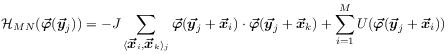
[65.2.0.6] On the mesoscopic level
the regularized block action representing the total configurational energy
of a single block (e.g. for block
.
[65.2.0.5] The partitioning introduced above allows two regularizations
into a lattice field theory.
[65.2.0.6] On the mesoscopic level
the regularized block action representing the total configurational energy
of a single block (e.g. for block ![]() ) reads
) reads
 |
(2.5) |
where ![]() denotes nearest neighbour
pairs of cells inside block
denotes nearest neighbour
pairs of cells inside block ![]() such that each pair
is counted once.
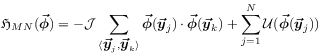
[65.2.0.7] On the macroscopic level one has the discretized action between blocks
(representing the total configurational energy)
such that each pair
is counted once.
[65.2.0.7] On the macroscopic level one has the discretized action between blocks
(representing the total configurational energy)
 |
(2.6) |
where now ![]() denotes nearest neighbour
blocks.
[65.2.0.8] Although the overall form of the discretizations is identical
for
denotes nearest neighbour
blocks.
[65.2.0.8] Although the overall form of the discretizations is identical
for ![]() and
and ![]() the macroscopic discretized fields
the macroscopic discretized fields
![]() and interactions
and interactions ![]() may in general require
renormalization in the infinite volume and continuum limit,
and are
therefore denoted by different symbols.
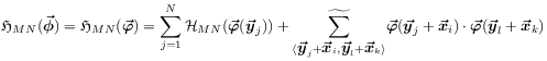
[65.2.0.9] Rearranging eq. (2.5)
the macroscopic discretized action
may in general require
renormalization in the infinite volume and continuum limit,
and are
therefore denoted by different symbols.
[65.2.0.9] Rearranging eq. (2.5)
the macroscopic discretized action ![]() is related to
the mesoscopic discretized action
is related to
the mesoscopic discretized action ![]() through
through
 |
(2.7) |
expressing a decomposition into bulk plus surface energies.
[65.2.0.10] Here
![]() expresses a summation over nearest neighbour
[page 66, §0]
cells
in the surface layers of adjacent blocks such that each pair of
adjacent block surface cells is counted once.
[66.1.0.1] Conventional field
theory or equilibrium statistical mechanics assumes that the surface
term which is of order
expresses a summation over nearest neighbour
[page 66, §0]
cells
in the surface layers of adjacent blocks such that each pair of
adjacent block surface cells is counted once.
[66.1.0.1] Conventional field
theory or equilibrium statistical mechanics assumes that the surface
term which is of order ![]() becomes negligible
compared to the bulk term which is of order
becomes negligible
compared to the bulk term which is of order ![]() in the
field-theoretic continuum limit.
in the
field-theoretic continuum limit.
II.B Fieldtheoretic scaling limit
[66.1.1.1] Consider now a scalar local observable![]() (composite operator) fluctuating from cell to cell.
[66.1.1.2] The fluctuations
generally define a correlation length
(composite operator) fluctuating from cell to cell.
[66.1.1.2] The fluctuations
generally define a correlation length ![]() whose magnitude
depends on the observable in question and the parameters
whose magnitude
depends on the observable in question and the parameters ![]() in the
Hamiltonian.
[66.1.1.3] The reconstruction of the continuum theory from its
discretization is usually carried out in two steps [24].
[66.1.1.4] First
one takes the (thermodynamic) infinite volume limit
in the
Hamiltonian.
[66.1.1.3] The reconstruction of the continuum theory from its
discretization is usually carried out in two steps [24].
[66.1.1.4] First
one takes the (thermodynamic) infinite volume limit
![]() at constant
at constant ![]() as the limit of canonical
(Boltzmann-Gibbs) probability measures in the finite volume.
[66.1.1.5] The
existence of this limit requires stability and temperedness of the
interaction potentials [25]. The limit amounts to setting
as the limit of canonical
(Boltzmann-Gibbs) probability measures in the finite volume.
[66.1.1.5] The
existence of this limit requires stability and temperedness of the
interaction potentials [25]. The limit amounts to setting
![]() and thus
and thus ![]() .
.
[66.1.2.1] Given the existence of the infinite volume limit one studies the
scaling limit ![]() of the regularized infinite-volume
theory.
[66.1.2.2] This field theoretic limit in general requires the
renormalization of the action
of the regularized infinite-volume
theory.
[66.1.2.2] This field theoretic limit in general requires the
renormalization of the action ![]() .
[66.1.2.3] The quantities
of main interest are the correlation functions
.
[66.1.2.3] The quantities
of main interest are the correlation functions
| (2.8) | |||
| (2.9) |
within a single block here chosen to be the one at the origin, i.e.
![]() .
[66.1.2.4] The normalization constant
.
[66.1.2.4] The normalization constant ![]() is the partition
function, the measure
is the partition
function, the measure ![]() is the finite volume lattice probability distribution on the space
of field configurations, and the notation
is the finite volume lattice probability distribution on the space
of field configurations, and the notation ![]() for the expectation value expresses its dependence on the parameters
in the Hamiltonian.
[66.1.2.5] The correlation functions (2.9) are
plagued the well known short distance singularities in the continuum
limit
for the expectation value expresses its dependence on the parameters
in the Hamiltonian.
[66.1.2.5] The correlation functions (2.9) are
plagued the well known short distance singularities in the continuum
limit ![]() .
[66.1.2.6] The standard approach [24] to this problem is
to keep
.
[66.1.2.6] The standard approach [24] to this problem is
to keep ![]() fixed and to use instead a lattice rescaling procedure
in which the auxiliary rescaling factor
fixed and to use instead a lattice rescaling procedure
in which the auxiliary rescaling factor ![]() diverges.
[66.1.2.7] This keeps the theory explicitly finite at all
steps.
[66.1.2.8] Thus the field theoretic continuum theory is defined through
the limiting renormalized correlation functions
diverges.
[66.1.2.7] This keeps the theory explicitly finite at all
steps.
[66.1.2.8] Thus the field theoretic continuum theory is defined through
the limiting renormalized correlation functions
| (2.10) |
where ![]() is the field renormalization.
[66.1.2.9] The parameters
is the field renormalization.
[66.1.2.9] The parameters ![]() approach a critical point
approach a critical point ![]() such that the
rescaled correlation length
such that the
rescaled correlation length
| (2.11) |
remains nonzero.
[66.2.0.1] The field theoretical continuum or scaling limit is called
“massive” or “massless” depending on whether the rescaled
correlation length approaches a finite constant or diverges to
infinity.
[66.2.0.2] Because ![]() is fixed equations (2.2) and
(2.11) imply
is fixed equations (2.2) and
(2.11) imply ![]() in the massive
scaling limit, and this allows to rewrite equation (2.10) as
in the massive
scaling limit, and this allows to rewrite equation (2.10) as
| (2.12) |
if the limit exists.
[66.2.0.3] In that case the renormalization
factor ![]() has the form
has the form
| (2.13) |
by virtue of the relation
| (2.14) |
which follows generally from renormalization group theory [26].
[66.2.0.4] Here ![]() is the anomalous dimension of the operator
is the anomalous dimension of the operator ![]() .
.
II.C Ensemble limit
[66.2.1.1] The ensemble limit introduced in [20] is a way of defining
infinite volume continuum averages from the discretized theory in a finite
volume without actually calculating the measure ![]() explicitly.
[66.2.1.2] The idea is to focus on the one point functions given by
(2.12) with
explicitly.
[66.2.1.2] The idea is to focus on the one point functions given by
(2.12) with ![]() as
as
| (2.15) | |||
| (2.16) | |||
 |
(2.17) |
where independence of ![]() by virtue of translation invariance
has been used in the first and the last equality.
[66.2.1.3] At criticality
these functions contain information about fluctuations through
the renormalization factor
by virtue of translation invariance
has been used in the first and the last equality.
[66.2.1.3] At criticality
these functions contain information about fluctuations through
the renormalization factor ![]() for field averages.
for field averages.
[66.2.2.1] For a given field configuration the fluctuating local
observable inside cell ![]() of block
of block
![]() will again be denoted by
will again be denoted by ![]() as defined above
and illustrated in Figure 1.
[66.2.2.2] The block variables
as defined above
and illustrated in Figure 1.
[66.2.2.2] The block variables
| (2.18) |
![]() are defined by summing the cell variables and the
ensemble variable
[page 67, §0]
are defined by summing the cell variables and the
ensemble variable
[page 67, §0]
| (2.19) |
is obtained by summing the block variables.
For ![]() the ensemble limit is defined as the limit
the ensemble limit is defined as the limit
| (2.20) |
where ![]() is a constant.
[67.1.0.1] In the ensemble limit
is a constant.
[67.1.0.1] In the ensemble limit ![]() as compared to
as compared to ![]() in the fieldtheoretic scaling limit.
[67.1.0.2] The difference to the field theoretic scaling limit is that
thermodynamic (
in the fieldtheoretic scaling limit.
[67.1.0.2] The difference to the field theoretic scaling limit is that
thermodynamic (![]() ), continuum (
), continuum (![]() ) and critical
(
) and critical
(![]() ) limit are taken simultaneously.
[67.1.0.3] In this way an infinite ensemble of regularized infinite classical
continuum systems is generated.
[67.1.0.4] The elements of the ensemble are
replicas of one and the same system governed by the Hamiltonian density
) limit are taken simultaneously.
[67.1.0.3] In this way an infinite ensemble of regularized infinite classical
continuum systems is generated.
[67.1.0.4] The elements of the ensemble are
replicas of one and the same system governed by the Hamiltonian density
![]() .
[67.1.0.5] Thus the ensemble limit generates an ensemble in the sense
of statistical mechanics.
.
[67.1.0.5] Thus the ensemble limit generates an ensemble in the sense
of statistical mechanics.
[67.1.1.1] The critical or noncritical averages ![]() can be calculated in the ensemble limit as
can be calculated in the ensemble limit as
| (2.21) |
[67.1.1.2] This equation states that macroscopic ensemble averages can either be calculated using equations (2.9) in the traditional scaling limit or directly using equations (2.18) and (2.19) in the ensemble limit. [67.1.1.3] Equation (2.21) gives the connection between the scaling limit and the ensemble limit. [67.1.1.4] Note that the validity of eq. (2.21) requires the existence of the renormalized field theory. [67.1.1.5] Thus the left hand side of (2.21) cannot be calculated at anequilibrium phase transitions [21, 22] while the right hand side can still be calculated in such cases.
| Type of scaling limit | |||||||
|---|---|---|---|---|---|---|---|
| 1. discrete ES limit | |||||||
| 2. | |||||||
| 3. massive scaling limit | |||||||
| 4. massless scaling limit | |||||||
| 5. massive FSS limit | |||||||
| 6. massless FSS limit | |||||||
| 7. continuum ES limit | |||||||
| 8. |
II.D Summary of different scaling limits
[67.1.2.1] The main difference of the ensemble limit as compared to other
scaling limits is that the three limits ![]() are simultaneously performed while in other limits only two of these
limits are taken simultaneously.
[67.1.2.2] There
are
are simultaneously performed while in other limits only two of these
limits are taken simultaneously.
[67.1.2.2] There
are ![]() ways of performing the scaling limit with the
three variables
ways of performing the scaling limit with the
three variables ![]() depending on whether a particular variable
is set equal to its limiting value or not.
[67.2.0.1] The different possibilities
are summarized in Table I.
[67.2.0.2] Note that only the ensemble limit (1.) and the related critical limit (7.)
in an infinite continuum theory yield an infinite number of uncorrelated
blocks.
[67.2.0.3] The close relation between the ensemble limit and the massive finite
size scaling limit (5.) is apparent if
depending on whether a particular variable
is set equal to its limiting value or not.
[67.2.0.1] The different possibilities
are summarized in Table I.
[67.2.0.2] Note that only the ensemble limit (1.) and the related critical limit (7.)
in an infinite continuum theory yield an infinite number of uncorrelated
blocks.
[67.2.0.3] The close relation between the ensemble limit and the massive finite
size scaling limit (5.) is apparent if ![]() .
.
